Source release: www.whatdotheyknow.com/request/earth_science_past_papers_and_ex/response/3419815/attach/4/Papers.zip?cookie_passthrough=1
For an approximately isotropic rock, the P wave and S wave speeds arewhere is bulk modulus, is shear modulus, and is density. Five important controls are:
- Mineralogy and cementation. Stiff, well-cemented mineral frameworks usually have higher elastic modulus values and faster seismic velocities than poorly consolidated sediments. Density alone is insufficient: both stiffness and density enter the equations.
- Porosity and cracks. Larger porosity, especially compliant cracks, usually lowers effective elastic modulus values and seismic velocities. Crack orientation can make the seismic velocities direction-dependent through seismic anisotropy.
- Pore-fluid composition and saturation. Replacing liquid water by gas generally lowers the effective bulk modulus sharply and reduces . Pore fluids have negligible static shear modulus; responds chiefly through the solid framework and the changed bulk density, rather than through a shear restoring force in the fluid.
- Effective confining pressure. Increasing effective stress closes cracks and improves grain contacts, usually increasing both seismic velocities. Increasing pore fluid pressure at fixed total stress reduces effective stress and can reverse this trend.
- Temperature. At otherwise comparable conditions, increasing temperature generally softens minerals and lowers seismic velocities; thermal cracking or partial melting can lower them further. Increasing burial commonly increases both temperature and pressure, so their separate effects need not have the same sign.
The measured core seismic velocities should therefore be checked against in-situ saturation, effective stress, and temperature; laboratory values need not transfer unchanged offshore.
The normal-incidence acoustic impedance is , with units . ThusDefine the pressure-amplitude reflection coefficient and pressure-amplitude transmission coefficient for incidence downwards from layer into layer byHere denotes compressional normal-stress amplitude; in the water it is the acoustic pressure. Continuity of normal traction and normal particle velocity gives these expressions. They describe each interface separately, before any layer layer reverberation.
For a lossless normal-incidence plane wave, intensity is proportional to , soA transmitted pressure amplitude exceeding unity is therefore compatible with conservation of energy. If instead the coefficient is defined for particle velocity measured along the same downward coordinate, and : the two transmitted velocity coefficients are and . Upward incidence reverses the sign of , interchanges the transmitted pressure and velocity coefficients, and leaves unchanged. At normal incidence between these ideal isotropic layers there is no P-to-S seismic mode conversion.
Take horizontal interfaces, water depth , and sediment thickness . Both source and receiver are just below the sea surface. Every angle below is measured from the vertical interface normal. Snell's law preserves the horizontal seismic ray parameterA basement seismic head wave of speed has horizontal propagation at the basement interface, so . The two possibilities are:
The water supports only P waves. At oblique incidence the seabed can convert a P wave into an SV-wave in the sediment, and the return SV-wave can convert back to a P wave in the water. Further seismic mode conversion can occur at the basement. Thus the down-going and up-going sediment legs can independently be P or S. The S entries refer to SV-waves; a fluid P wave source in this two-dimensional isotropic geometry does not excite the decoupled SH-wave sector.
Let be the distance travelled along the basement interface. For sediment legs ,The first-appearance distance is the limiting value at :
For example, the unconverted P branch gives . The earliest geometrically permitted basement P seismic head wave is the doubly converted path with sediment S legs, at approximately . The corresponding basement S family first appears at approximately . These limiting distances describe existence of ray branches; a finite detectable wave amplitude also depends on conversion efficiency and acquisition noise.
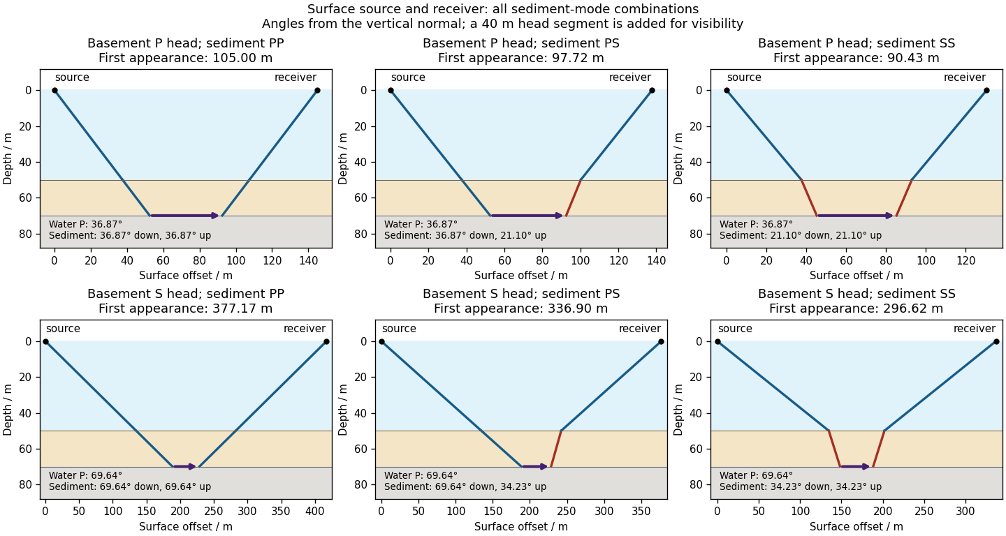

There is no separate finite-distance P head wave at the water–sediment interface: , so the nominal critical angle is , and a ray from a source 50 m above the interface cannot reach it at finite horizontal distance. Nor can the slower sediment S speed, , support a seismic head wave launched from water: it would require . A seismic reflection still exists at the seabed because the densities, hence the acoustic impedances, differ.
First appearance and first arrival differ. For each permitted branch the travel time isThe all-P basement P branch has . It overtakes the direct water P wave, , only at . The converted P-head branches have larger seismic intercept times, so even where they exist at shorter offsets they are later arrivals. The S-head branches are likewise later than the all-P P-head branch wherever they exist in this model. Reflections and layer reverberations can supply additional later phases.
Use a high-resolution multichannel seismic reflection survey, with closely spaced crossing lines or a suitable small three-dimensional survey over the turbine locations. It should map the seabed, the sediment–sandstone boundary, local faults, buried channels, and lateral changes relevant to foundations. Seismic reflection responds to acoustic impedance contrasts and can image an irregular boundary without requiring it to be a first-arrival refractor. Here even the seabed has a useful normal-incidence reflection coefficient of despite its zero P-velocity contrast.
A seismic refraction survey can provide complementary seismic velocities and geotechnical information, particularly using seabed multicomponent receivers for S waves. Its limitations as the principal imaging method here include the missing water–sediment P refractor, required offsets of hundreds of metres to obtain useful basement first arrivals, and weaker constraints on thin layers or velocity inversions. Variable bathymetry and sediment thickness further complicate simple refraction interpretations.
A shallow-towed boomer seismic source or small sparker seismic source is a sensible initial seismic source for penetrating about 20 m of sediment beneath a 50 m water column. A chirp sub-bottom profiler can add finer imaging of the upper cover where penetration permits; penetration depends on grain size, consolidation, gas, and seismic attenuation. A pilot line should establish the minimum useful source energy and bandwidth. Large low-frequency air-gun arrays are unnecessary for this shallow target. Small coastal vessels, sea state, tow stability and acoustic background constrain usable frequencies and operations. Marine mammals and other local receptors motivate a low-energy effective source, monitoring and appropriate operational mitigation.[ref]
High-resolution multichannel seismic system by United States Geological Survey. The institutional instrument description lists configurable boomer, sparker, hydrophone-streamer and complementary chirp equipment for shallow subsurface mapping.
The expected normal-incidence two-way travel times are for the seabed and for basement, separated by . Source duration, recording sample interval and bandwidth must distinguish them. As an initial vertical seismic resolution estimate, : gives about in the sediment, although usable resolution depends on the whole seismic wavelet and signal-to-noise ratio.
Choose shot and receiver spacing from the shortest useful wavelength, target size, maximum reflector dip, seismic migration needs and achievable navigation accuracy. For a plane event of horizontal seismic ray parameter , avoiding spatial aliasing requires approximately . Source spacing and receiver spacing also set midpoint coverage and seismic acquisition fold; adequate offsets enable moveout correction and velocity estimation. For nearly horizontal shallow reflectors a few-metre shot interval can be practical, whereas steep events at high frequency require denser spatial sampling. These values must be designed together rather than imposing one spacing for every target. Cross-line spacing must resolve lateral features between turbine sites, not merely along each track.
At a vessel speed of , one shot per second gives 2 m shot spacing and ample separation relative to a roughly target return, subject to the longer record needed for seismic multiples and source recovery. Shallow towing limits seismic source ghosts and receiver ghosts, but requires stable tow depth. Accurate positioning, tides, measured water sound speed, bathymetry and checks for seabed seismic multiples are essential for correct target depths.
A gravity anomaly is the difference between observed gravitational acceleration and a specified reference prediction after defined reductions. A free-air gravity anomaly, a Bouguer gravity anomaly, and a residual local gravity anomaly differ because they remove different reference contributions. State the reference ellipsoid, datum, reference density, and regional trend before interpreting an anomaly as a subsurface geophysical density contrast.
On land, tie gravimeter observations to a gravity base, calibrate them, correct instrumental drift and Earth tides, and determine station latitude and elevation accurately. Subtract latitude-dependent normal gravity . Reduce to the reference elevation using a positive free-air correction for a station above that datum: about for in metres. A simple Bouguer gravity anomaly then subtracts attraction of the intervening rock slab and adds the conventional terrain correction:with all acceleration terms expressed consistently. In SI units .
At sea, also correct vessel-motion effects, especially the Eötvös correction from east–west vessel motion and Earth rotation, and vertical ship acceleration; average or filter the moving-platform data appropriately. GPS navigation and tide information specify position and measurement height. Sea-surface measurements give a marine free-air gravity anomaly after motion, latitude, tide and height reductions. A marine Bouguer gravity anomaly additionally allows for measured bathymetry and the replacement of low-density water by reference rock; the simple water-column replacement correction is positive, , relative to the sea-surface free-air value. A consistent three-dimensional bathymetric correction is preferable near irregular coasts. Remove a justified broad regional field if the intended quantity is a residual anomaly of the local body.
For a wide horizontal Bouguer slab replacing surrounding basement, use the density contrast , not the absolute sediment density:Take downward attraction as positive. The negative anomaly therefore requires . With , , and ,soThis is the requested Bouguer slab approximation: a flat observation surface, laterally infinite constant-thickness material, uniform average geophysical density contrast, and a regional anomaly already removed. The actual basin in Figure 1 narrows downwards and is finite. For a fixed maximum thickness, finite width reduces the central anomaly magnitude, so this calculation can underestimate the true magnitude of the average geophysical density contrast. It does not establish a unique basement density without the geometrical assumption.
Use the same surrounding basement density inferred in solution, carrying its unrounded value through the arithmetic. The intrusion's geophysical density contrast isThe Bouguer slab thickness needed to produce the same negative peak is thereforeThe smaller absolute geophysical density contrast requires a thicker body. This is an approximate vertical thickness and, if the top is close to the surface as drawn in Figure 1, an approximate base depth below that top. It is not an independent estimate of the intrusion's burial depth. For an infinite slab the anomaly does not depend on top depth; a buried top would require additional geometry. Finite width and the downward-widening outline in Figure 1 make 8 km a slab-equivalent estimate rather than a uniquely determined geological depth.
For the two negative gravity anomalies in the actual Figure 1, examine where the steepest flanks occur within the total fall into the trough. The solid upper intrusion profile has maximum slope relatively low on its flanks, close to the flat trough; its body widens downwards. The lower basin profile has maximum slope relatively high on its flanks, near the shoulders; its body narrows downwards. The dashed gradient traces and arrows mark these transitions. The signed derivative changes sign on opposite sides of a symmetric trough; a plot of gradient magnitude instead gives two positive peaks.
A shallow edge controls a relatively abrupt local change, whereas deeper geophysical density contrast spreads its effect over greater horizontal distance. Downward-narrowing geometry leaves relatively more of the anomaly associated with the shallow broad part, placing the strong flank change nearer the outer shoulders. Downward-widening geometry adds a broader deep contribution beneath the narrow outcrop, shifting the inflection towards the lower part of the trough. Thus the location of a flank's maximum slope relative to its shoulder and minimum is more useful here than the shared peak alone.
A symmetric constant-density body with vertical sides gives a symmetric negative trough with paired rounded flanks; for a broad shallow body the main slope changes occur approximately halfway down those flanks. It is intermediate between the two end members, rather than a triangular anomaly or a rectangular discontinuity. Exact fractional inflection heights depend on width, depth, burial and rounding. The following independently calculated infinite-strike models illustrate the distinction without copying Figure 1.
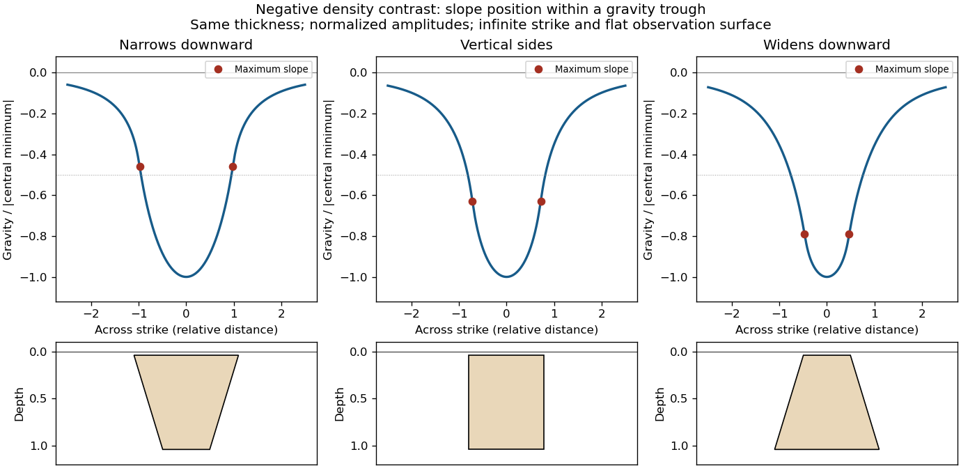

This qualitative inference assumes approximately comparable simple bodies, uniform geophysical density contrast, and a properly removed regional field. Gravity inversion is non-unique: lateral density changes, multiple bodies, and a buried top can imitate changes of wall slope. Use the seismic reflection constraints to test the interpretation.
Assume that the intrusion has a positive magnetic susceptibility contrast, that induced magnetization dominates its remanent magnetization, and that the local present-day geomagnetic field points roughly northward and downward, as in this northern mid-latitude setting. Writewhere is the anomalous magnetic field and the last expression assumes . A total-field magnetic anomaly measures a field projection, so it need not have the same sign everywhere above a high-susceptibility body.[ref]
The 100 km east–west extent makes an approximately two-dimensional, east–west-striking body a useful model away from its ends. On a profile drawn north on the left, south on the right, the expected normally induced response has a subsidiary negative lobe on the northern side and a stronger positive lobe over the body, displaced towards the south. The northward horizontal field component makes the anomaly asymmetric; its downward component produces the dominant positive response. The field falls back towards the regional value away from the intrusion. Broad bodies can have edge shoulders or a broad central high, so the sketch represents a qualitative shape rather than one uniquely specified curve.
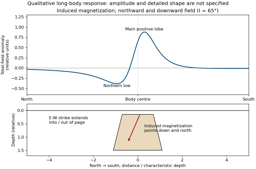

An exactly vertical inducing field would remove this north–south skew for a symmetric induced body. Real magnetic inclination and magnetic declination should be taken from a suitable geomagnetic field model for the survey date and location; no exact local value is supplied here. Strong oblique or reversed remanent magnetization can shift or reverse the lobes, and heterogeneous magnetic susceptibility, body dip and three-dimensional end effects can alter the profile. Higher magnetic susceptibility alone does not determine a unique amplitude or polarity pattern without these qualifications.
Use compression-positive principal stresses, . For the intended thrust fault regime during approximately north–south tectonic shortening, the likely orientations areA locally horizontal traction-free surface motivates taking one principal direction as vertical, while the strong north–south compression selects the maximum horizontal principal stress. The expected fault strike is then approximately east–west.
This ordering assumes the two horizontal compressions exceed the vertical principal stress. North–south shortening by itself does not establish the magnitudes of all three: if the vertical principal stress were intermediate, strike-slip faulting would instead be possible. The answer above is the simple compressional end member used in the following parts.
A reverse or thrust fault earthquake is the expected end member: a hanging wall moves upwards relative to its footwall, accommodating north–south tectonic shortening. A plausible double-couple seismic source focal mechanism has an approximately east–west fault strike, a moderately north- or south-dipping fault plane, and up-dip fault slip. For example, right-hand-rule strike , southward fault dip about , and fault rake specify a pure thrust mechanism.
In a lower-hemisphere equal-area plot, with shaded regions denoting compressional P first motions, this focal mechanism has a shaded central region and two unshaded outer lobes. The P axis is approximately horizontal north–south and the T axis approximately vertical for a symmetric idealization; for a single plane their axes are slightly tilted. The P and T axes of a double-couple seismic source need not exactly equal the regional principal stress axes. The nodal curves represent both the fault plane and its auxiliary plane; additional evidence is needed to choose between them.[ref]
Focal mechanisms or beachballs by United States Geological Survey. Lower-hemisphere compression shading and the ambiguity between the two nodal planes.
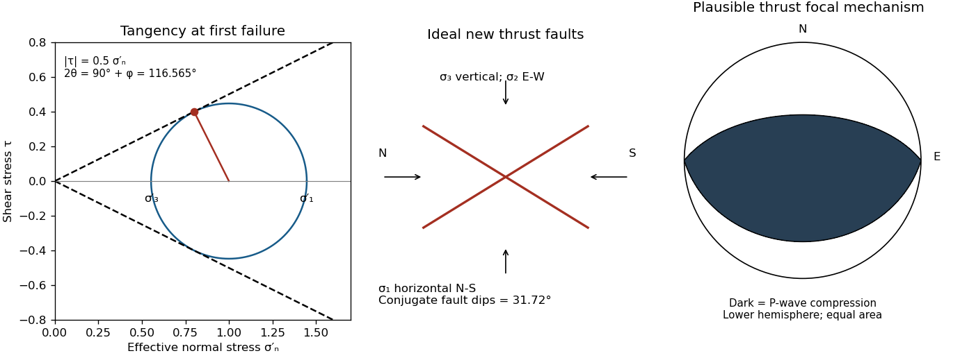

Assume an initially unfractured homogeneous isotropic material described by a linear Mohr-Coulomb failure criterion, with the given coefficient of friction representing the relevant internal friction angle. Use spatially uniform pore fluid pressure, effective stresses , and compression-positive signs. ThenThe Mohr circle in the plane has centre and radius . At first failure it is tangent to the failure envelope. The radius to the positive-shear tangent point is perpendicular to the line of slope , hence makes angle with the positive normal-stress axis.
If is the angle between the fault normal and , the stress transformation isThus , , and the angle of the fault itself to horizontal isThe two conjugate thrust faults therefore strike approximately east–west and dip about north and south. This is the fault dip, not the fault-normal angle. Both sediments and basement have the same optimum orientation under these assumptions because their stipulated friction slopes are equal; their cohesion and absolute failure stresses could still differ.
The first two panels in solution give the labeled construction. Constant cohesion shifts the straight failure envelope without changing its slope, and uniform pore fluid pressure translates the Mohr circle in normal-stress coordinates; neither changes this tangency angle. In the illustrative cohesionless case, , giving . Pre-existing weaknesses, a nonuniform stress field, anisotropic strength, or a nonlinear failure envelope invalidate the simple optimum-orientation prediction.[ref]
Stress and strength lecture notes by MIT OpenCourseWare. Lecture 10 develops the traction, pore-pressure and Mohr-circle framework; the signs and angle definitions above specify the convention used here.
The result predicts initial failure in a uniform material under the assumed principal-stress orientations. The actual Figure 3 is a present-day NW–SE cross section through a thick, heterogeneous Alpine stack, extending to about 50 km depth. It contains near-horizontal basal stretches, curved ramps, tightly bent contacts, and steep structures in the internal zones around Viso and the Dora Maira complex. It does not show a single undeformed conjugate pair newly formed in horizontal uniform rock.
Several processes explain the departures:
- Mechanical layering and inherited weaknesses. Faults can follow weak bedding, old fault planes, or contacts with lower friction or cohesion than the surrounding rock. These can form shallow décollements linked by steeper ramps. Figure 2 explicitly distinguishes the near-surface red “geophysical bedrock” boundary at a few hundred metres from the much deeper crystalline basement beneath the Jurassic, Triassic and Permian cover. An age label or a seismic contrast alone does not establish a friction coefficient; clay-rich or evaporite detachments are possibilities to test, not lithologies proved by that drawing.
- Rotation after formation. Continuing tectonic shortening, folding, stacking and fault slip can rotate an initially optimal fault plane to steeper or shallower present-day fault dips. A steep older structure may be inherited from an earlier deformation episode rather than created at its present orientation.
- Curved faults and local stresses. Faults bend through a layered crust; local principal stress axes rotate near topography, ramps and interacting faults. The optimum angle is measured relative to the local , not necessarily to the regional horizontal direction everywhere.
- Changing strength and deformation mechanism. Spatial changes in pore fluid pressure, coefficient of friction, cohesion and temperature alter which surfaces reactivate. At depth, ductile deformation can replace frictional brittle failure, so the same new-fracture construction need not apply throughout the section.
Finally, a section shows apparent dip unless it is perpendicular to fault strike. For an ideal plane, , where is the angle between the section direction and fault strike. Obliquity can make a plane look shallower, but cannot on its own explain an apparent dip steeper than its true dip. Do not infer that each black curve is a currently active brittle earthquake fault.
The northern station is closer, under comparable P wave and S wave paths through the same velocity model. In the actual Figure 4 the northern P and S pulses are separated by about 6 s, whereas the southern separation is roughly 8–8.5 s. The S–P time removes the unknown earthquake origin time:Both northern pulses also occur earlier on the shared absolute clock, consistent with the smaller distance. Earlier arrival alone would not be sufficient if clocks or velocity models differed.
For reproducible graph readings, the northern positive-to-negative zero crossings are approximately for P and for S; the southern crossings are approximately and . These are convenient corresponding pulse landmarks, not sharply defined first-break onsets. The first visible motion begins earlier: approximately 12 s and 18 s in the north, and 14–15 s and 22–23 s in the south, depending on the amplitude threshold. The horizontal axis is seconds since midnight on 1 January 2000, not elapsed time since rupture initiation.
Use the northern S–P time, approximately , rather than multiplying an absolute-clock arrival by a wave speed. For common approximately straight paths,No numerical crustal velocities are specified in Q3. If the usual illustrative crustal values and are adopted, the distance isThese assumed crustal speeds are unrelated to Q1's offshore layer values. They are representative rather than measurements of the Swiss column; the British Geological Survey gives broad typical crustal ranges of 5–7 km/s for P waves and 3–4 km/s for S waves.[ref]
How are earthquakes detected by British Geological Survey. The seismic-wave table provides typical crustal speed ranges, not a velocity model for this particular earthquake.
Using the corresponding northern central pulse times gives an effective source time near after midnight, and the S estimate is the same to graph accuracy. The southern central landmarks similarly give a distance near 70 km and an effective source time near 5 s. That consistency supports the example, but pulse landmarks need not mark the rupture's true onset. is a source-to-station path or hypocentral distance in the uniform-speed approximation. An epicentral distance additionally needs the hypocenter depth; it cannot simply be equated to 50 km for an unknown depth.
Distinguish the duration of one phase pulse from the P-to-S separation. Figure 4 shows northern pulses with most visible motion over roughly 3–4 s each, compared with roughly 4–5 s or more in the south. Reading the low-amplitude tails gives approximately 11.5–15.2 s for the northern P pulse, 17.7–20.9 s for the northern S pulse, 14.2–19.0 s for the southern P pulse, and 22.3 s to beyond the right plot boundary near 27 s for the southern S pulse. Thus the latter duration is censored by the plotting window; it should not be assigned an exact ending at 27 s. The positive-to-negative extremum separations are only about 1 s in the northern pulses, 1.3 s in the southern P pulse and 1.4 s in the southern S pulse; those much shorter numbers are not full source durations. Smooth tails have no unique onset or ending at the precision of this drawing.
A finite-source rupture has an intrinsic duration that differs from the apparent pulse duration through rupture directivity. In an ideal unilateral line-source model, neglecting local slip rise time, instrument filtering and path broadening,Here is the chosen phase wave speed and is the rupture's projection along equal-and-opposite takeoff directions. Averaging corresponding full pulses in that model suggests an intrinsic timescale of roughly 4–5 s. This is an order-of-magnitude graph estimate, not an exact rupture duration; the figure does not supply a seismic source time function definition, receiver responses, phase deconvolution, or geometry sufficient to determine one uniquely. A finite local slip rise time would also contribute to the observed width.
In particular, neither 13 s nor 19 s is a rupture duration: those numbers locate phase motion on the absolute clock. The northern P–S gap of 6 s is a propagation delay rather than the rupture duration.
For a unilateral finite-source rupture advancing at approximately constant rupture velocity , the along-fault propagation length isThere is no supplied or calibrated seismic source time function, so a unique spatial extent cannot be read directly from Figure 4. For illustration, and an assumed would give . Allowing – and assumed – gives lengths of order 8–15 km. These are explicitly conditional scale estimates, not measured fault dimensions.
If equal-and-opposite ray geometry and phase pulse durations were known, the directivity model in solution would instead constrain a projected length,where is the angle between the rupture direction and the northern ray. Distinct P and S wave speeds, unknown takeoff angles, smooth pulse boundaries and the clipped southern S tail prevent a reliable independent numerical inversion here. This observation is consistent with a few-kilometre projected extent while the actual along-fault length can be larger. A rupture length is not the accumulated fault slip, the width of the whole fault plane, or the approximately 50 km station distance.
The shorter, stronger northern pulses and broader southern pulses suggest propagation from south to north, towards the northern station. The useful evidence is the difference in pulse widths, not just the earlier northern arrivals: the latter chiefly reflect station distance.
As rupture reaches successively more northerly patches, each patch radiates a new P wave and S wave pulse. Towards the north, the later emission time is partly cancelled by a shorter propagation path; those contributions arrive closer together. Towards the south, later emission and a longer path add, stretching the signal. This is rupture directivity. It refers to the advance of the slipping region along the fault, not necessarily the direction of the local fault slip vector. A thrust can slip up-dip while its rupture front advances in a direction with a northward component.
More generally, emission from a patch at distance along the rupture arrives atThe forward direction has a smaller arrival-time spread. This is the same travel-time compression captured by isochrone-based rupture directivity calculations.[ref]
A formulation of directivity for earthquake sources using isochrone theory. The primary report relates directivity to rupture geometry, seismic speed and the arrival-time distribution of radiation from successive fault patches.
Larger northern amplitude supports the interpretation but is not decisive on its own because geometrical spreading, seismic attenuation, seismic radiation patterns and site response also affect amplitude. With only two traces, propagation, filtering and site effects remain alternatives to test; the idealized exercise is most naturally explained by northward directivity.The geomorphology of active normal faulting records a competition between accumulated tectonic displacement and the ability of erosion, transport and deposition to modify it. A hanging wall moves down relative to a footwall, producing a fault scarp, mountain-front relief, and accommodation space for a sedimentary basin. Repeated earthquakes can build a large front even though each individual surface break is much smaller.[ref]
Normal-fault geomorphic features by United States Geological Survey. The primary mapping report's table of geomorphic features lists scarps, faceted spurs, oversteepened mountain fronts and rejuvenated valley floors as common normal-slip indicators.
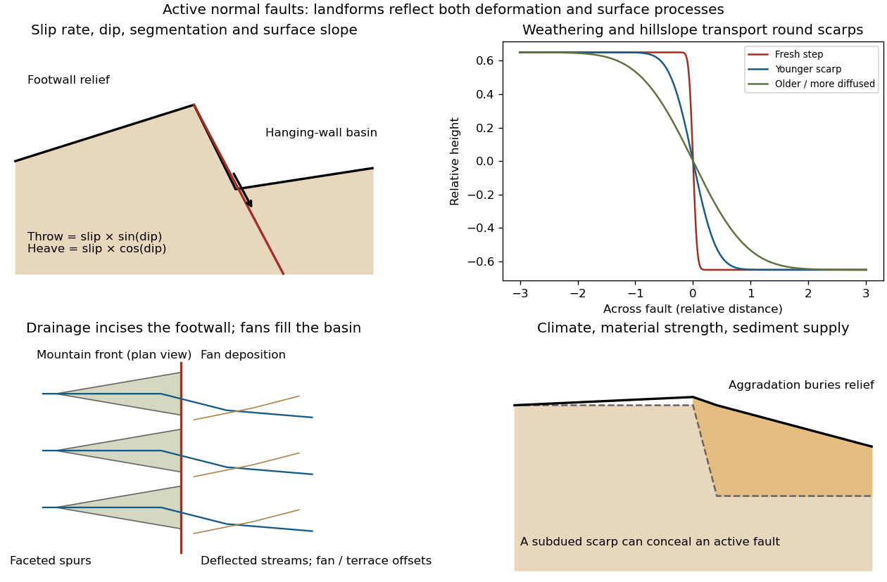
Original sketches of tectonic, erosional and depositional controls on normal-fault landforms
. The panels distinguish cumulative block displacement, progressive scarp rounding, drainage and faceted mountain fronts, and burial of a scarp by sediment. Geometries and relative scales are illustrative. Details.
The principal controls and their observable effects are:
- Displacement, rate and timing. Larger single-event fault slip creates a higher fresh scarp; repeated slip builds cumulative offsets of fans and river terraces. The interval since the latest rupture controls degradation. For pure dip-slip faulting on a plane dipping , vertical fault throw is and horizontal fault heave is . Scarp height on an inclined eroded surface need not equal either the slip or the original vertical throw.
- Geometry and structural history. Fault dip, strike, curvature, segmentation, splays and along-strike variations in fault slip control scarp orientation and continuity. Linked faults can create a stepped front; synthetic and antithetic faults can create a graben. Cumulative deformation includes broad footwall uplift and hanging-wall tilting as well as a sharp break.
- Lithology and cover. Strong exposed bedrock can preserve steep scarps and fresh fault surfaces. Weak fractured rock, thick regolith and loose alluvium weather and slump more rapidly, spread deformation, and produce debris at the scarp base. Differential erosion can make a lithological front without recent tectonic movement, so a straight cliff alone is not sufficient evidence of activity.
- Climate and surface transport. Rainfall, runoff, frost action, vegetation and slope processes control scarp rounding and colluvium production. Steep new faces collapse towards stable slopes; later hillslope transport rounds the crest and fills the toe. A simple scarp diffusion model broadens a step over a length proportional to , but only if a suitable transport law and comparable material and climate apply.
- Drainage and sediment supply. Footwall uplift can incise channels and produce river terraces, knickpoints and triangular faceted spurs. Hanging-wall subsidence can pond drainage, deflect streams and promote alluvial fans and basin filling. Rapid aggradation can bury an active scarp, while stream incision can remove or exaggerate local relief.
- Preservation and initial landscape. Pre-existing slopes, relief, surface ages, glacial modification and human disturbance determine where offsets can be recognized. A fan abandoned long before the latest earthquake can accumulate more offset than a younger nearby surface. Compare like-age markers across a fault, and distinguish a mountain front's long history from a single event.
Useful observations therefore include scarp profiles, repeated offsets of dated surfaces, drainage organization, and continuity along strike. A high rugged front is not by itself evidence of a high present fault slip rate; conversely, a muted or buried scarp need not mark an inactive fault.
A surface-reaching normal fault earthquake commonly produces a down-facing step towards the hanging wall, accompanied by extension across the break. A fresh free face can expose bedrock, polish or striations, roots or offset soil. The actual rupture is usually irregular: fault slip changes along strike, separate strands overlap or step, and tension fissures, small grabens and secondary cracks distribute part of the extension.
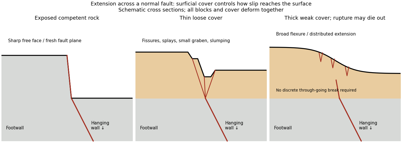
Original cross sections showing how surficial cover changes normal-fault surface rupture
. Competent exposed rock localizes a sharp free face; thin loose cover permits splays and a small graben; thick weak cover can accommodate a buried fault tip by broad flexure and distributed extension. Details.
Exposed competent rock or very thin cover: a relatively narrow, sharp break can closely follow the principal fault plane. A steep free face can be recognizable immediately, then weather and shed debris. The face need not be vertical or maintain the same height along strike.
Loose granular or poorly consolidated cover: the main shear can splay upwards through alluvium or regolith. Open fissures, step-like scarps, rotated blocks, synthetic and antithetic normal faults, and a small intervening graben can form across a wider zone. Collapse and raveling quickly build colluvium at the toe. A single rupture event can therefore create several parallel breaks; counting them does not count earthquakes.
Thick weak or cohesive cover: deeper fault slip can be transferred into distributed shear strain, tilted beds, broad warping or monoclines, with tension cracks above a propagating tip. A discrete break may be attenuated or absent if the fault remains blind. Cover thickness alone is not enough to predict the response: cohesion, grain size, layering, saturation, rupture displacement and fault depth also matter. Saturated loose sediment can additionally develop soil liquefaction, sand blows or lateral spreading; these are secondary shaking effects and do not independently locate the tectonic rupture.
The observed vertical step, crack aperture and total width of disturbed ground should be measured separately. Reconstruct the total displacement across all strands and account for the original ground slope. Landslides or gravitational spreading can imitate normal-fault scarps, so map connections to the main fault and displaced markers rather than assuming every open crack is primary tectonic slip.
Excavate across the mapped fault scarp, approximately perpendicular to its strike, at a site where young sediments record and preserve deformation. On cleaned trench walls log bedding, soil horizons, shear zones, fissure fills, buried surfaces and colluvial wedges. Correlate the same marker beds across the fault before reconstructing individual displacements.
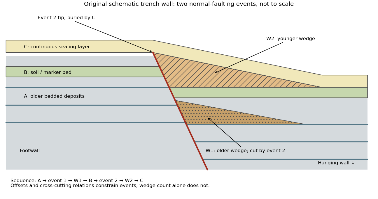

- A fault or fissure cuts older layers but terminates below an undeformed sealing deposit. The event occurred after deposition of the youngest demonstrably displaced material and before deposition of the oldest demonstrably sealing material.
- A fresh free face sheds coarse angular debris, often thickest against the scarp and thinning into the hanging wall; later finer slopewash can overlie it. A buried soil horizon between successive colluvial wedges can indicate a period of stability separating events. Fissures filled from above can preserve collapsed soil blocks or distinctive younger sediment.
- Older markers may have larger offsets than younger markers. A lower wedge or soil cut and displaced by a younger shear, then overlain by a new wedge and an intact seal, gives a cross-cutting basis for at least two events. Changes in displacement should be reconstructed across all fault strands.
- Rapid tilting, growth of accommodation space, abrupt changes in deposit thickness, and locally ponded beds can corroborate the structural evidence. Soil liquefaction structures or shaking-induced landslides may support a chronology, but do not alone prove surface rupture on the trenched fault.
In the drawing, A was faulted in event 1; W1 accumulated; B buried and stabilized that surface. Event 2 displaced A, W1 and B, after which W2 accumulated and C sealed the fault tip. Thus A records two events, B one and C none. This combination of offset and sealing relationships is stronger evidence than identifying two wedge-shaped units alone.
Bracket event ages with multiple samples just below and above the event horizons. Suitable short-lived organic material can be dated by radiocarbon dating; optically stimulated luminescence dating can constrain deposition of appropriate mineral grains. Reworked old charcoal, younger roots, incomplete bleaching, erosional gaps and time elapsed between rupture and wedge deposition must enter the age interpretation. For calendar dates, only when those deposits genuinely bracket the rupture; a radiocarbon age in years before present reverses the numerical ordering.[ref]
Introduction to paleoseismology by United States Geological Survey. “Finding Paleoearthquakes” explains disrupted layers followed by unbroken cover; “Determining the Age of a Paleoearthquake” explains dating deposits above and below the event horizon.
One earthquake can generate several debris pulses and wedges; repeated earthquakes may reuse one strand without leaving separable deposits. Erosion, bioturbation, nondeposition, lateral facies changes and upward-dying splays can hide events or mimic terminations. Confirm relationships on both trench walls and, when possible, in adjacent exposures. The result is a minimum supported event sequence with age intervals, not an assumption of perfectly periodic recurrence or one earthquake per wedge.
Put and suppose , so there are interior grid points , . Write . The fixed ends impose homogeneous Dirichlet boundary conditions,For a sufficiently smooth displacement field, the two Taylor series at fixed time givewhere all displayed derivatives on the right are evaluated at . Adding cancels the odd terms, leaving the second-order central differenceSubstitute this finite difference into the wave equation and retain continuous time. The resulting method of lines gives coupled second-order ordinary differential equations,In particular, the first and last equations are and for . With the interior displacement vector only,Equivalently, , , and all other entries vanish. This entrywise definition also covers small , including when . The matrix is a symmetric matrix and a tridiagonal matrix. The spatial approximation has error in Big O notation; time has not yet been discretized.
For a nonzero, time-independent vector , substitute . Taking two time derivatives givesCancel the nonzero exponential to obtain the eigenvalue problemThus an eigenvector specifies a normal mode shape and its negative eigenvalue specifies the square of its angular frequency, . Real displacements are obtained by taking the real part, or by combining the two temporal solutions as .
The interior grid is , with fixed-end displacements . HenceUse the monic characteristic polynomial convention , where is the identity matrix. Expansion of the determinant along the first row givesThe eigenvalues are the roots of a polynomial . With the alternative determinant convention , the characteristic polynomial is because the matrix has odd size; its roots of a polynomial are unchanged.
For each row, a Gershgorin disc has centre and radius . Here and , so the Gershgorin circle theorem givesSince is a real symmetric matrix, its eigenvalues are real. Intersecting the union of these Gershgorin discs with the real axis yieldsThis bound permits zero but does not assert a zero eigenvalue. The fixed-end Dirichlet boundary conditions exclude it: for any nonzero real vector , extend by and calculateIndeed, equality would force every adjacent value to agree with the zero endpoint. Thus is a symmetric positive-definite matrix, is a negative-definite matrix, and the eigenvalues satisfy . The same argument works for any number of interior grid points, with prefactor in the sum. The fixed string has no zero-frequency rigid translation.
Each supplied eigenvector gives relative displacements at in a standing wave. Insert zero at to describe the whole sampled string. A real normal mode is : its shape stays fixed while its amplitude oscillates.
- is the highest-frequency resolved normal mode. Adjacent interior displacements alternate in sign: the middle point moves opposite to both outer interior points. Its interpolated shape has three lobes, corresponding to the third string normal mode.
- is the middle-frequency normal mode. The midpoint is a node of a standing wave, and the two sides move in opposite directions. It corresponds to the second string normal mode.
- is the lowest-frequency normal mode, corresponding to the fundamental frequency. All interior points move in the same direction, with greatest displacement at the centre; the only nodes of a standing wave are the endpoints in the smooth shape through these samples.
These semidiscrete fixed-string normal modes are samples of , with in the order listed. More precisely, their interior vectors are , which have unit Euclidean norm and form an orthonormal basis of . Their eigenvalues and angular frequencies obeyThus larger absolute value of a negative eigenvalue means faster oscillation, rather than faster decay. The numerical angular frequencies approximate the continuous fixed-string values ; the finite difference spatial approximation changes them. Only three independent interior normal modes exist on this grid, and any interior displacement or initial velocity vector can be expanded in this orthonormal basis.
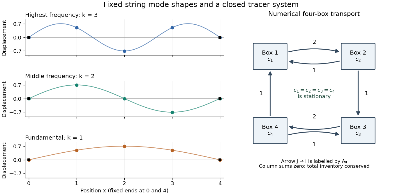

Apply Gaussian elimination to the supplied nonsymmetric matrix,The first pivot element is , with elimination multiplier . Perform , givingThe second pivot element is , with elimination multiplier . Perform , then use the third pivot element and elimination multiplier to perform . The LU factorization isHere is a unit lower triangular matrix, hence an invertible matrix, and is an upper triangular matrix. No row interchange is needed: all three pivot elements used in elimination are nonzero. The final diagonal entry is zero, with an entirely zero last row; there is no further division by it. The three nonzero rows of are linearly independent, so the matrix rank is and is a singular matrix. Direct matrix multiplication gives .
Since is an invertible matrix, is equivalent to . The last nontrivial row gives ; the second gives ; and the first gives , so . A basis of the null space is thereforeIts single basis vector has Euclidean norm , so the unit null space basis vector is .
The pivot elements of lie in columns . Take these columns from the original matrix to obtain a basis of its column space:The fourth column is minus the sum of these three columns, and the leading three-by-three matrix minor has nonzero determinant , confirming linear independence.
Elementary row operations preserve the row space. Thus the nonzero rows of give a basis of the row space of :These basis vectors need not have unit Euclidean norm or be orthogonal. Their Euclidean norms are , respectively; the three column basis vectors have Euclidean norms .
Regard as a linear map . By the rank-nullity theorem and matrix rank ,All three are vector subspaces of , with the row space identified with four-component row vectors in the usual way. The null space lies in the input vector space of concentrations; the column space lies in the output vector space of concentration-change rates. Both have four coordinates, although they play different physical roles.
In this particular matrix, the row sums and column sums both vanish. Put . Then and , and the two three-dimensional vector subspaces coincide:This equality follows here from both sum identities and the dimensions of a vector space; it does not make a symmetric matrix and is not true for every square matrix.
The null space consists of concentration patterns on which transport produces no change. Here it is the familyEvery box has the same concentration. Ocean circulation may continue, but inflow and outflow of the chemical tracer balance in each box. With these are exactly the steady states; physically admissible members have . With nonzero , adding to any particular steady state leaves its transport balance unchanged, but a null space vector alone need not balance the sources and sinks.
To identify the tracer inventory, apply conserved inventory from a left null vector. Directly summing each column givesConsequently, for the supplied ordinary differential equations,For , is a conserved quantity. The connected box model equalizes concentrations, approaching the unique member of the null space with the initial inventory:The arithmetic mean is appropriate here because the supplied matrix has zero column sums. In a general box model the conserved quantity is , where is a positive left null space vector; for physical concentrations expressed per unit volume, these weights represent the box volumes up to a common factor. One must establish the weights from the equations, rather than infer equal volumes from a schematic drawing.
Nonnegative initial concentrations remain nonnegative under transport alone. Indeed is a nonnegative matrix, sohas nonnegative entries for : it is a positive matrix semigroup. Its column sums are one by . To see why equalization occurs, set for ; then andThe right side vanishes only for constant , which in the zero-sum vector subspace means . Its strict negative bound on the unit sphere in that vector subspace gives decay to zero. Thus the matrix exponential redistributes inventory without creating negative concentrations; arbitrary prescribed sinks can still exhaust the tracer if they are allowed to act indefinitely.
A steady state satisfies , henceThe sign is positive on the right after rearranging the supplied equation. A solution exists exactly when lies in the column space of , which above was found to be the zero-sum vector subspace. Equivalently, multiply by the left null space vector :This condition is necessary and sufficient for an algebraic steady state, since both the column space and that zero-sum vector subspace have dimension . It expresses global conservation of mass: in the closed box model, total tracer production must balance total tracer removal. With the paper's convention , a positive is a sink and a negative is a source. If the sum is nonzero, and the inventory changes linearly in time, preventing a steady state.
When the condition holds, all algebraic steady states form the affine solution space of a linear equation , for any particular solution . The initial inventory selects one member through . For a physically admissible solution, its four concentrations must additionally be nonnegative; the compatibility condition alone imposes no such inequalities.
Choose a fixed time increment , let , and approximate by . The Backward Euler method evaluates the transport term at the new time:Rearrange to the linear systemAlthough is a singular matrix, is an invertible matrix for every . In each row, its diagonal entry is and the sum of the absolute values of its off-diagonal entries is ; hence it is a strictly diagonally dominant matrix. Its Gershgorin discs have centre and radius , excluding zero. In particular, the zero eigenvalue of becomes an eigenvalue of .
- Form once. Compute a Pivoted LU decomposition , storing the permutation matrix , the unit lower triangular matrix , and the upper triangular matrix .
- Set .
- At each step form . Solve by forward substitution, then solve by back substitution.
- Advance and repeat until the desired final time. Choose the fixed increment so the final time is an integer multiple of , or refactor if a shorter final step is used.
Both triangular solves use the factors of . The LU factorization of the singular transport matrix from part (a) is not a solver for this new linear system. No matrix inverse needs to be formed. Since and are fixed, the same LU factorization serves every step; only the right-hand side changes. A varying would give without changing these factors.
As a check, multiplying the update by givesexactly reproducing the inventory balance at the sampled times, apart from roundoff error. The Backward Euler method has temporal global error for smooth solutions, so its A-stability does not remove the need to select for accuracy.
Set and . If , the integrand is one and its integral is . If is a nonzero integer,ThusThis is Fourier orthogonality in its unconjugated form. With a complex conjugate on the second exponential, the nonzero case would instead be .
Multiply the complex Fourier series by and integrate over one period. Fourier orthogonality removes every term except the one with index , givingFor general square-integrable functions, this is an orthogonal projection onto the corresponding Fourier mode. It remains valid when the expansion converges only in L2 space: integrate finite Fourier partial sums first, then pass to the limit using the Cauchy-Schwarz inequality. No unjustified pointwise exchange of an infinite series and an integral is needed.
The displayed signal is a square wave with levels and , each lasting two seconds. On a representative period it is positive for and negative for .
The waveform repeats after one positive and one negative interval, so its fundamental period is . A two-second shift reverses its sign and is not a period.
The zero Fourier coefficient is . For a nonzero integer , integrate the two constant halves:ConsequentlyThe complex Fourier series is . The negative-index coefficients are the complex conjugates of the positive-index ones, as required for a real signal. Combining each pair gives the equivalent real expansionAt a jump, pointwise convergence of a piecewise smooth Fourier series gives zero, the average of the two one-sided limits. The value assigned to at isolated jumps does not affect its Fourier coefficients or mean-square signal power.
The squared signal equals except at irrelevant isolated jump times. Its mean-square signal power is thereforeHere “power” has the signal-processing definition specified in the question. To convert this voltage mean square into electrical power in watts, a load electrical resistance would also be required: .
Use Parseval identity for Fourier series with the coefficient normalization above. Only odd nonzero indices contribute; summing the positive and negative indices givesThusThe factor of two from the negative frequencies is essential. The discontinuities do not obstruct Parseval's identity, which is a statement about L2 space.
Most of the mean-square signal power lies at low frequencies. Each nonzero coefficient has magnitude , so its power contribution decreases as . The pair at the fundamental frequencies alone containsof the total. The first three positive odd harmonics, together with their negative-frequency partners, contain about . The harmonic power of a square wave still has a nonzero tail: higher harmonics are needed to reproduce sharp edges even though their combined power is small.
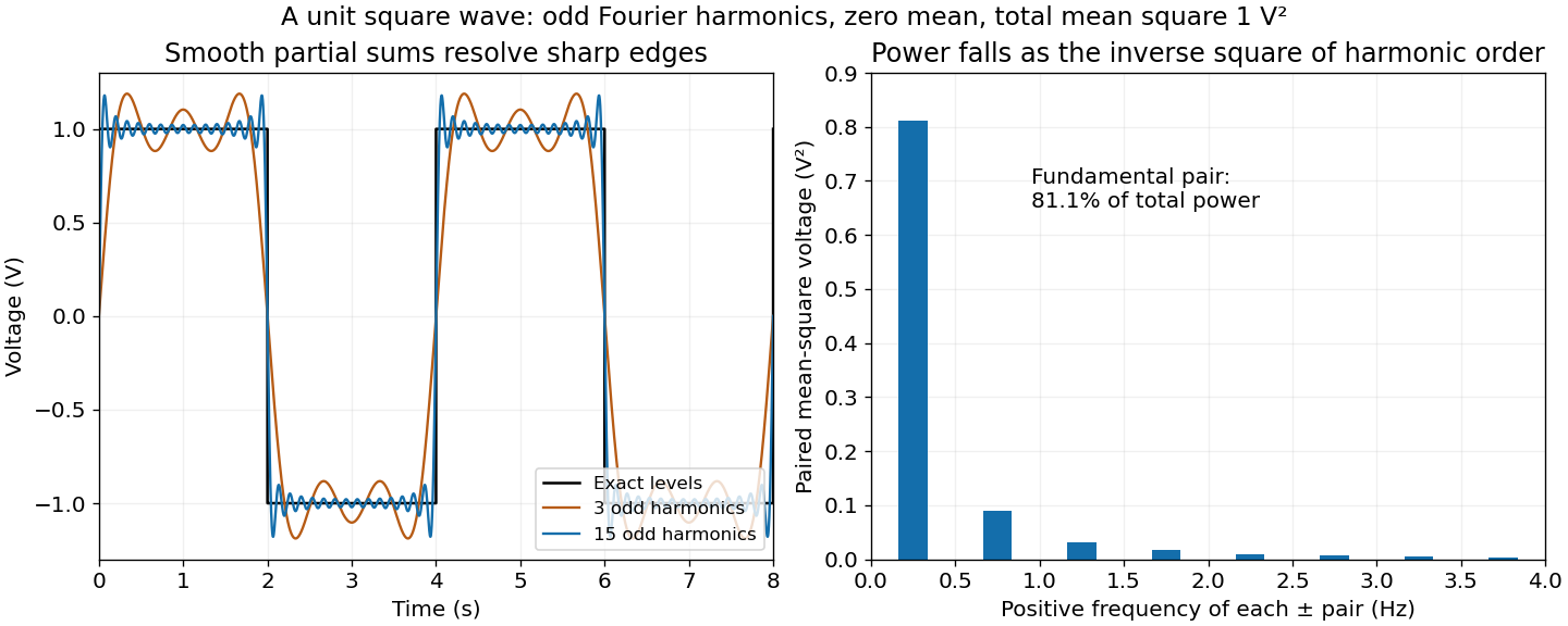

Apply a Fourier transform or discrete Fourier transform, retain the desired low-frequency coefficients and attenuate those in the high-frequency noise band with a low-pass filter, then invert. For a real signal, apply matching gains at positive and negative frequencies to preserve Hermitian symmetry.
Parseval identity for Fourier series shows what an ideal coefficient cutoff does: the output mean-square signal power is the sum of the retained squared coefficients, and cannot exceed that of the unfiltered input. Much of the high-frequency noise can be removed, but a finite cutoff also removes genuine square wave harmonics. Its edges become less sharp, and a sharp spectral cutoff can exhibit the Gibbs phenomenon. There is no claim of exact recovery if the noise overlaps the retained band. Noise already folded into low frequencies by aliasing cannot in general be removed merely by discarding the high-frequency bins afterward.
Articles were limited to the first 100 out of 141 total.
Articles by others on the same topic
There are currently no matching articles.