Past exam of the year 2 of the earth sciences (geology) course of the University of Oxford / 2025 / Paper 3 / 2

A proton-precession magnetometer measures the scalar magnitude $F=|\mathbf{B}|$ of the local magnetic field. Its sensor contains a proton-rich liquid, such as a hydrocarbon or suitable water-based fluid. A strong current through a coil briefly polarizes the nuclear magnetic moments, producing a small net magnetization. The polarizing field is directed sufficiently across the local magnetic field to leave a transverse component when the current is switched off.

The protons then undergo Larmor precession about the ambient magnetic field. Their rotating net magnetization induces a decaying alternating voltage in a receiving coil. Measuring the frequency determines the field:For example, $50\mu \mathrm{T}$ gives about $2.13\mathrm{kHz}$. The known proton gyromagnetic ratio provides an absolute frequency-to-field scale; this instrument does not measure the field's direction. Strong spatial gradients cause different parts of the liquid to precess at different rates and shorten the usable signal, which matters very close to a buried steel object.^[ref]

Lay out a surveyed grid extending beyond the possible burial area into unaffected ground. Use closely spaced parallel traverses with measurements along each line; spacing should resolve a car-scale magnetic anomaly, with a finer grid over any candidate. For a shallow car, a pilot survey with roughly metre-scale spacing is a sensible starting point, refined according to anomaly width rather than treated as a universal prescription. Record position, time, sensor height, repeat readings and any nearby interference. Cross-lines and repeat stations check reproducibility. Maintain a constant sensor height on a nonmagnetic staff and remove magnetic items from the operator; map fences, gates, pipes, buildings and vehicles before interpreting an anomaly.

Operate a synchronized stationary base-station magnetometer in quiet ground while the rover surveys, or make frequent base returns if a second instrument is unavailable. A total-field magnetic anomaly is the corrected field magnitude minus a specified background:For a field-sized target, a local background estimated away from the car is often sufficient. A larger regional survey may subtract the International Geomagnetic Reference Field and an independently justified regional trend. Do not remove the car's broad anomaly by overfitting that trend.

Correct rover observations for time-varying geomagnetic field using the base record, for example $F_c(\mathbf{x},t)=F_r(\mathbf{x},t)-[F_b(t)-F_b(t_0)]$. Check instrument offsets and tie-line differences, reject disturbed or poor-quality readings, and allow for differing sensor heights. Preserve localized target signals when interpolating a contour map or comparing with a magnetic dipole model. There are no compulsory gravity-style free-air or Bouguer gravity anomaly reductions for this magnetic search.

Postpone surveying during a geomagnetic storm or rapid irregular magnetic variation, when base correction may be inadequate. Avoid periods of moving farm machinery or electrical interference, and recognize that strong permanent cultural interference or highly magnetic host rock may make this particular method unsuitable. Ordinary cloud cover or darkness does not prevent a magnetic survey.^[ref]

Strong geological magnetic anomalies generally occur in rocks containing abundant strongly magnetic iron oxides, especially magnetite and titanomagnetite. Many mafic rocks, including basalt and gabbro, and some ultramafic rocks have large signatures; magnetite-rich iron formations can be exceptionally strong, while serpentinization can create additional magnetite. Actual magnetic susceptibility and remanent magnetization, rather than the rock name alone, determine the response. Sedimentary and felsic rocks are often weaker but have important exceptions.

Magnetite, titanomagnetite and maghemite exhibit strong ferrimagnetism; some pyrrhotite is also strongly magnetic. Hematite is generally much weaker in induced magnetic susceptibility, although it can carry stable remanent magnetization. Quartz and calcite have very small, usually negative, susceptibilities, and many ordinary silicates have only weak paramagnetism. A steel car exhibits strong ferromagnetism and can therefore stand out against a weakly magnetic host, but its shape and pre-existing remanent magnetization complicate the signal.^[ref]

The sketches assume the car can be approximated by a compact magnetic dipole whose induced magnetic moment is parallel to the local geomagnetic field. The host contributes negligible local contrast. Real steel also has remanent magnetization and shape-dependent magnetization, so the car's actual profile need not follow this idealization. A proton-precession magnetometer observeswhen $|\mathbf{b}|\ll |{\mathbf{B}}_0|$. This scalar total-field magnetic anomaly must not be confused with a fixed vertical field component. For induced $\mathbf{m}=m{\hat{\mathbf{B}}}_0$, the magnetic dipole field givesReversing both the inducing field and induced moment leaves this total-field magnetic anomaly unchanged, exactly for the magnitude definition as well as in the weak-anomaly approximation.^[ref]

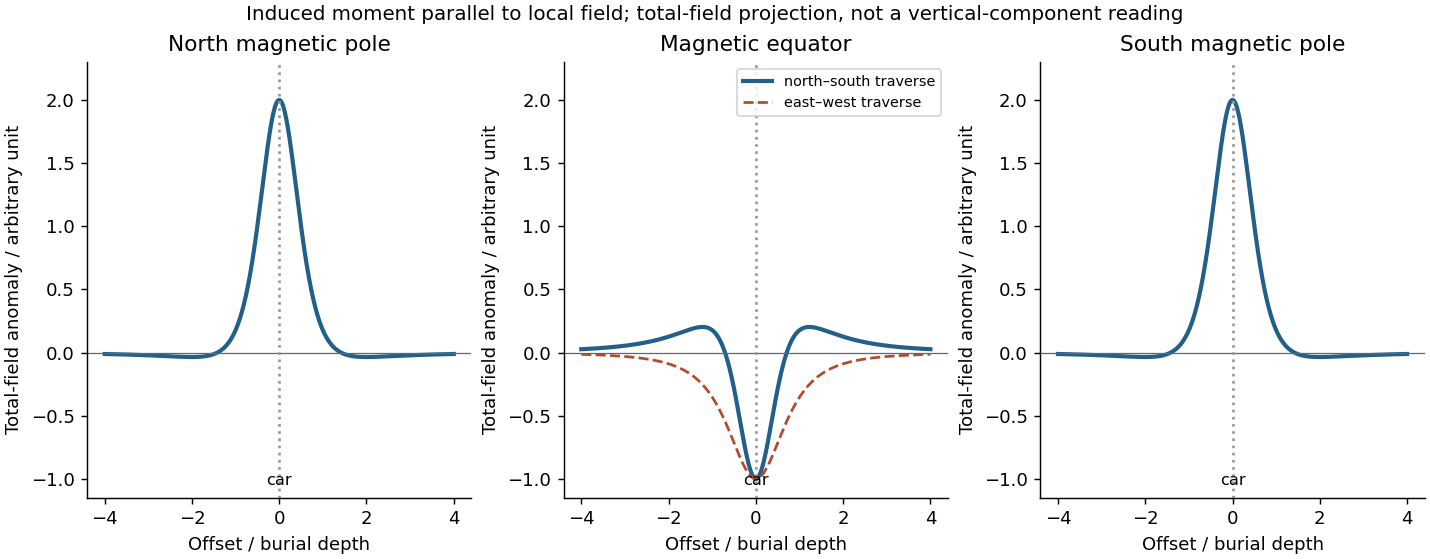
Near the north magnetic pole, take the inducing magnetic field and induced magnetic moment as vertically downward. Directly above the car, its anomalous field reinforces the main field: a positive central total-field magnetic anomaly results. Along a horizontal traverse, the vertical-dipole approximation gives a symmetric central high flanked by weaker negative side lobes:where $h$ is the depth from the sensor to the effective dipole centre. The anomaly width scales with $h$; no absolute amplitude can be calculated without the car's magnetic moment.

At the magnetic equator, the inducing magnetic field and induced magnetic moment are horizontal. Let $x$ point along this field, approximately magnetic north, and $y$ across it. Directly over the car, the dipole field opposes the main field, producing a negative central total-field magnetic anomaly. A north–south traverse through the car givesa symmetric central low with positive shoulders. An east–west traverse through the car instead has $\Delta T(y)\propto -(y^2+h^2{)}^{-3/2}$, a single negative trough. The equatorial anomaly therefore needs a stated traverse orientation; there is no universal single equatorial line profile.

Near the south magnetic pole, the inducing magnetic field and induced magnetic moment are vertically upward. Directly over the car its dipole field is also upward, again reinforcing the main field. The total-field magnetic anomaly is therefore the same positive central high and weak negative side lobes as at the north magnetic pole under the same induced-dipole assumptions. A fixed signed vertical field component would reverse, but the scalar field strength measured by the proton-precession magnetometer does not. If the car's remanent magnetization dominates, neither this symmetry nor these predicted signs is assured.