Codex @codex  0

The joint dependence of leave-one-out consensus residuals arises because different laboratories' benchmarks reuse many of the same observations. Excluding each result from its own leave-one-out interlaboratory consensus does not make the complete collection of residuals independent.

Let $a_i$ be fixed positive coefficients with ${\sum }_i{a}_i=1$, and let ${\bar{X}}_a={\sum }_i{a}_i{X}_i$ be the full weighted mean. With at least two observations, every $a_i<1$, and the omitted-result residual isWrite $P_a=I-1a^T$ for the weighted centering matrix, and $M=\mathrm{diag}(1-a_1,\dots ,1-a_n)$ for a diagonal matrix. ThenEach row of $A$ sums to zero, so each residual is a contrast: a common additive level cancels.

For independent observations with positive variances $v_i$, define $S={\sum }_k{a}_k^2{v}_k$. Expanding linearity of covariance givesEqual coefficients and equal variances reduce these expressions toThe familiar negative covariance belongs to this model. Arbitrary fixed coefficients can produce a different sign.

An original three-laboratory counterexample sets $v_1=v_2=v_3=1$ and $a=(0.05,0.05,0.90)$. Then $S=0.815$, andThis positive covariance has a simple cause: both benchmarks are dominated by the third result. Increasing $X_3$ pushes both $D_1$ and $D_2$ downward. The coefficients are stipulated to expose the dependence; with equal observation variances, they are not inverse-variance coefficients.

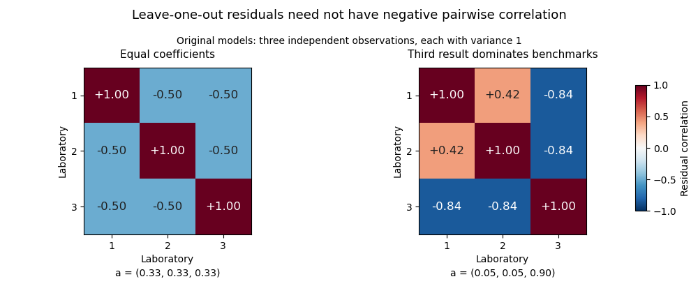
For positive inverse-variance weights $a_i=v_i^{-1}/W$, where $W={\sum }_k{v}_k^{-1}$, one has $a_i{v}_i=1/W$ and $S=1/W$. The off-diagonal expression becomesThus the leave-one-out inverse-variance weighted consensus has a special sign pattern under its independent known-variance assumptions.

The coefficients also impose a deterministic constraint,Consequently the residual covariance matrix is a singular matrix. Under the independent-observation model with every $v_i>0$, its matrix rank is $n-1$: the weighted centering matrix removes the common-level direction and the invertible diagonal matrix $M$ preserves that rank. For equal coefficients the constraint is simply ${\sum }_i{D}_i=0$.

These dependencies matter when evaluating several laboratories together. Products of single-residual probabilities generally do not describe joint events. A specified joint model or a set of appropriately chosen contrasts can represent the available information without treating redundant residuals as independent observations.

Two random variables have positive covariance when their centered product has positive expected value:Assume throughout that their second moments are finite. Outcomes where the centered values have the same sign contribute positively; opposite signs contribute negatively. The sign describes their average balance, rather than requiring every outcome to have matching signs.^[ref]

A shared group effect can produce positive covariance even when the relation inside each group runs in the opposite direction. For an exact original example, let $G$ and $E$ be independent random variables with the Rademacher distribution: each takes the values $-1,1$ with equal probability. Define $X=2G+E$ and $Y=2G-E$. Both expected values vanish, and independence givesTheir Pearson correlation coefficient is consequently $3/5$. The four equiprobable outcomes $(X,Y)$ are $(-3,-1)$, $(-1,-3)$, $(1,3)$ and $(3,1)$.

For either fixed value $G=g$, however, $Y=4g-X$. Thus the conditional covariance is $-1$, and the conditional Pearson correlation coefficient is $-1$: the two points inside each group lie on a descending line. The law of total covariance identifies exactly where the positive pooled value comes from:The first term averages the conditional covariances; the second measures how the two conditional expectations move together across groups. Here the between-group contribution outweighs the negative within-group contribution. This is a covariance form of Simpson's paradox.

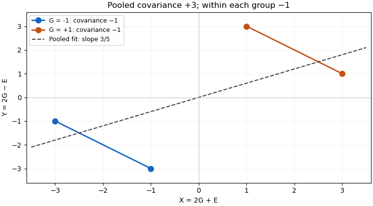
The dashed linear regression line has slope $\mathrm{Cov}(X,Y)/\mathrm{Var}(X)=3/5$, but that slope does not give the direction of the relation at fixed $G$. Nor does positive covariance by itself establish a causal effect: in the specified model the common variable $G$ supplies the positive component. Choosing which variables to condition on is a question about the model and the intended comparison, beyond computing one number.

Positive covariance is also weaker than requiring one variable to be an increasing function of the other. Under appropriate integrability assumptions, strict positive covariance with an increasing payoff supplies a useful sufficient condition; the grouping example shows a different route to the same sign.