Weighted arithmetic mean (${\bar{x}}_w$)

The weighted arithmetic mean combines values according to how much each contributes to the quantity being summarized. For a finite list of real numbers $x_i$ and nonnegative weights $w_i$ with $W={\sum }_i{w}_i>0$, defineZero weights ignore an entry; at least one weight must be positive. Multiplying every weight by the same positive number leaves the result unchanged. Writing $p_i=w_i/W$ makes the weighted mean a convex combination, since $p_i\ge 0$ and ${\sum }_i{p}_i=1$. It therefore lies between the smallest and largest input values. ^[ref]

For example, give the values $90$ and $60$ weights $2$ and $8$:The larger weight pulls the result closer to $60$. The balancing identityexplains a geometric interpretation: if the weights were masses placed at positions $x_i$, the weighted mean would be their center of mass. Here $8(66-60)=2(90-66)=48$, so the two sides balance even though their distances from the mean differ.

Weights need an interpretation. They can represent numbers of observations, masses, or probabilities in a finite probability distribution. These meanings lead to the same formula, while answering different questions. For instance, combining means of groups uses group sizes as weights to recover the mean over individual observations. For a function $f$ and nonnegative weight function $w$, the analogous integral is $\int wf/\int w$, provided $wf$ is integrable and the total weight $\int w$ is positive and finite.

Inverse-variance weighting combines estimates of the same quantity by giving a more precise estimate a larger weight. Suppose $X_i$ are independent, unbiased estimators of $\theta$, with known variances $0<{\sigma }_i^2<\infty$. For normalized weights,The inverse is taken after squaring the standard uncertainty: twice the standard uncertainty gives one quarter as much weight. The corresponding weighted least squares criterion is ${\sum }_i(X_i-\theta {)}^2/{\sigma }_i^2$; differentiating it with respect to $\theta$ gives the same weighted arithmetic mean.^[ref]

The optimality statement is precise. Any linear unbiased estimator ${\sum }_i{a}_i{X}_i$ requires ${\sum }_i{a}_i=1$. By the Cauchy-Schwarz inequality,Equality holds for the displayed weights. Thus they minimize variance among linear unbiased combinations under these assumptions; a normal distribution is not needed for that proof.

For an original example, combine observed values 10 and 14 with standard uncertainties 1 and 2 in the same units. The normalized weights are $0.8$ and $0.2$, giving estimate $10.8$, variance $0.8$ and standard uncertainty approximately $0.894$. Equal weights give 12 and standard uncertainty $\sqrt{1.25}\approx 1.118$.

Correlated errors change the problem. A contribution common to every reading survives every weighting whose coefficients sum to one; precision limits of weighting correlated repeats derives the resulting floor. More generally, use the full covariance matrix and generalized least squares rather than treating correlated readings as independent.^[ref] Uncertainty in estimated inverse-variance weights is another limitation: variances estimated from the same data are not fixed known quantities, and an accidentally tiny estimated variance does not justify arbitrary confidence.

Uncertainty in estimated inverse-variance weights arises when the variances used in inverse-variance weighting are themselves estimated. A very small estimated variance can give one observation or group a large random weight. The familiar variance formula for fixed, known weights cannot simply be reused with estimated variances treated as exact. NIST specifically warns that weights estimated from few replicates can substantially and unpredictably affect a weighted least squares analysis.^[ref]

Suppose independent groups contain $n_i$ independent normal random variables with common mean $\theta$ and group variance ${\sigma }_i^2$. Let ${\overline{X}}_i$ and $S_i^2$ be the group sample mean and unbiased sample variance, and formFor normal samples, each sample mean is independent of its sample variance. Conditional on the estimated weights, the estimator remains unbiased and hasThus the law of total variance gives unconditional variance equal to the expectation of this expression. The true ${\sigma }_i^2$ still appear; replacing them by the same random $S_i^2$ does not establish the actual conditional variance. Outside the independence assumptions, even conditional unbiasedness can fail.

An original two-group example takes $n_1=n_2=5$ and true ${\sigma }_1^2={\sigma }_2^2=4$, so each group mean has variance $0.8$. If observed sample variances are $0.25$ and $4$, the estimated normalized weights are $16/17$ and $1/17$. For group means $10$ and $14$, the combined estimate is $174/17\approx 10.2353$. The plug-in variance isbut the true conditional variance under the stipulated model isThe corresponding standard deviations are about $0.2169$ and $0.8435$. Equal weights would have variance $0.4$. An accidentally small estimated variance has both overstated precision and moved the combination away from the optimal equal weights in this example.

Reciprocal moments of an estimated variance explain the unstable precision estimate. For a normal sample with $\nu =n-1$, $Z=\nu S^2/{\sigma }^2$ has a chi-squared distribution. Integrating its density givesConsequently $\mathbb{E}[1/S^2]=\nu /[(\nu -2){\sigma }^2]$ for $\nu >2$, while the second moment requires $\nu >4$. The density and its gamma-distribution parameterization are documented in the primary SciPy implementation notes.^[ref] With $n=5$, the inverse sample variance has a finite mean twice the true precision and an infinite variance; the normalized weights remain bounded, so this does not imply their variance is infinite.

More replication or a justified smooth variance model can stabilize weights. NIST describes direct replicate-based weight estimation and variance-function modeling as distinct approaches.^[ref] A proposed validation repeats the complete weight-estimation and combination procedure on simulated or replicated groups, checking actual interval coverage as well as point estimates. A bootstrap must reproduce the weight-estimation stage; holding the fitted weights fixed tests a different procedure.

Reciprocal moments of an estimated variance determine whether a precision estimate such as $1/S^2$ has a finite expected value or variance. Small positive values of a sample variance become large values after inversion. An unbiased estimator of a variance therefore need not give an unbiased or even integrable estimate of its reciprocal.

For $n\ge 2$, let $X_1,\dots ,X_n$ be independent normal random variables with common mean $\mu$ and variance ${\sigma }^2>0$. For the unbiased sample variance $S^2=(n-1{)}^{-1}{\sum }_i(X_i-\overline{X}{)}^2$, put $\nu =n-1$. Then $Z=\nu S^2/{\sigma }^2$ has a chi-squared distribution. Its probability density function is $z^{\nu /2-1}{e}^{-z/2}/[2^{\nu /2}\Gamma (\nu /2)]$ for $z>0$.^[ref]

For any real $p>0$, direct integration and the Gamma function giveThe convergence restriction is essential: near zero the integrand has exponent $\nu /2-p-1$, so the integral diverges when $\nu \le 2p$. Substitution of a negative Gamma function argument into the displayed quotient does not define a nonexistent moment.

Rescaling gives the useful general resultIn particular, the mean reciprocal exists for $n>3$, while its variance requires $n>5$:For $n=6$ the mean is $5/(3{\sigma }^2)$, the variance is $50/(9{\sigma }^4)$ and the coefficient of variation is $\sqrt{2}$. For $n=4$ the mean is finite but the variance is infinite. For $n=3$ even the mean diverges. Increasing the number of groups does not repair a nonexistent moment of each raw reciprocal estimate.

Inverse-variance weighting commonly normalizes these reciprocals. Those normalized weights lie between zero and one, so their moments can exist even when the raw reciprocal moments fail. This distinction matters in uncertainty in estimated inverse-variance weights: neither the moment calculation nor a plug-in precision formula alone establishes the accuracy of the final weighted estimator. The results here use the exact normal-sample law; a nonnormal sample requires a different analysis.

For positive mean density, this average weights a velocity by local mass rather than volume. It satisfies the exact identity $⟨\rho u⟩=⟨\rho ⟩\tilde{u}$, so it naturally represents mass flux in averaged conservation laws. The ordinary volume mean generally fails that identity when density and velocity are correlated. Applied inside a phase, the same construction uses density times that phase's indicator as its weight.

For a partition of a set of complete sample observations into groups of known sizes $n_g$ and total $N$, its sample mean is the weighted mean of the group sample means. Indeed, dividing ${\sum }_g{\sum }_{i\in g}{y}_i={\sum }_g{n}_g{\overline{y}}_g$ by $N$ proves the identity. If the printed group means $m_g$ each have absolute rounding error at most ${\delta }_g$, their compatible pooled mean lies inThis follows because all the weights are nonnegative. Equivalently, the pooled absolute rounding error is at most ${\sum }_g(n_g/N){\delta }_g$, by the triangle inequality. A printed overall mean must have a rounding interval intersecting this interval. Disjoint intervals prove incompatibility, rather than merely a difference of displayed decimals. This is a necessary consistency check for means of the same complete sample; it cannot silently equate a full-sample mean with a different complete-case mean or establish a unique repair to inconsistent output.

Suppose disjoint nonempty groups have sizes $n_j$ and arithmetic means ${\bar{x}}_j$. The arithmetic mean of all observations isEach group contributes the sum $n_j{\bar{x}}_j$; add those totals before dividing by the overall count. This is exactly a weighted mean of group means with weights equal to group sizes. ^[ref]

Take a synthetic example with two observations equal to $90$ and eight equal to $60$. The two group means are $90$ and $60$, and the combined mean is $66$. Giving the two groups equal weights instead produces $(90+60)/2=75$, which summarizes the two group means with equal influence. To summarize all ten individuals with equal influence, use their group counts.

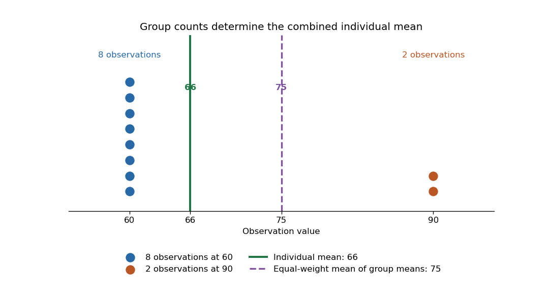
The group means and counts determine the combined arithmetic mean, but do not generally determine the combined variance. Variation within the groups is additional information.

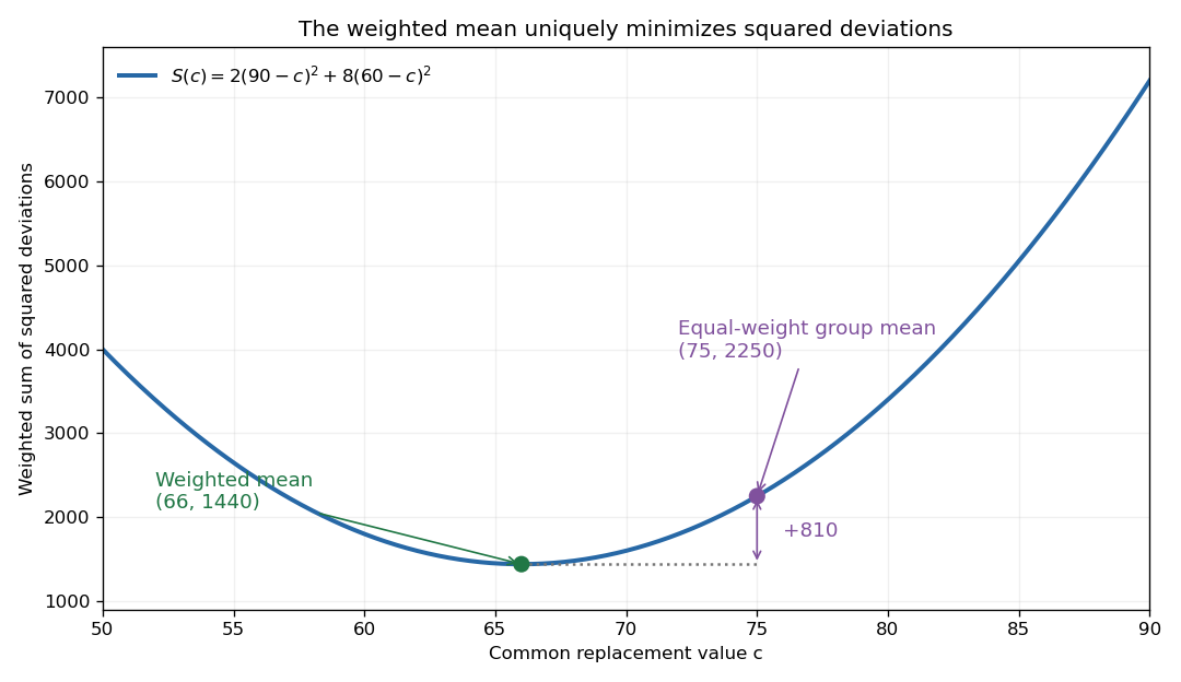
For a finite list of real numbers $x_i$ and nonnegative weights of positive total $W$, the weighted mean uniquely minimizes the weighted sum of squared deviationsExpanding around ${\bar{x}}_w$ and using ${\sum }_i{w}_i(x_i-{\bar{x}}_w)=0$ givesEvery displacement from the weighted mean increases the objective. This is the simplest one-parameter weighted least squares problem: represent all entries by one common value.

For the weighted values $90$ and $60$ with weights $2$ and $8$,Thus $S(66)=1440$, while $S(75)=2250$. The minimum is defined by this squared-error criterion; a different loss can select a different summary, such as a median under unweighted absolute deviations.

For a nonempty finite list of real numbers $x_1,\dots ,x_n$, the arithmetic mean isIt is the weighted mean with equal weights, giving each observation equal influence. For $(2,4,9)$, the sum is $15$ and the arithmetic mean is $5$. Replacing every value by $5$ retains the same total. The residuals $-3,-1,4$ sum to zero, so the mean is also the balancing point of these equally weighted observations.

The arithmetic mean minimizes the sum of squared deviations by the weighted mean minimizes squared deviations identity with all weights one. A large input can consequently have a substantial effect: replacing $9$ by $90$ changes the mean to $32$, while the median remains $4$. The choice of summary depends on what aspect of the data matters.

The harmonic mean of a nonempty finite list of positive real numbers is the multiplicative inverse of the arithmetic mean of their inverses:For two inputs, $H=2x_1{x}_2/(x_1+x_2)$. Replacing each input by $H$ preserves the sum of inverses, making it useful when a fixed amount divided by a rate determines a cost or duration. This positive-input definition avoids division by zero; negative inputs need not retain the usual averaging or ordering properties. ^[ref].

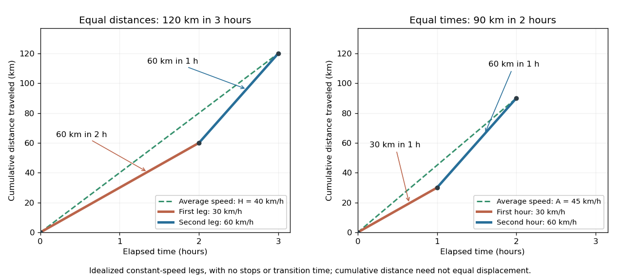
Travel two legs of equal length $d$ at positive speeds $v_1,v_2$, with no stops. Their travel times are $d/v_1$ and $d/v_2$, so the average speed isFor two $60\mathrm{km}$ legs at $30$ and $60km/h$, the times are two hours and one hour. The average speed is $120/3=40km/h$. The same speeds maintained for one hour each instead cover $90\mathrm{km}$ in two hours, giving the arithmetic mean $45km/h$. A slower equal-distance leg occupies more time, so the data being averaged must include what is held equal. This is total distance traveled divided by elapsed time; a return journey can have zero average velocity while keeping a positive average speed. ^[ref].

The arithmetic-geometric mean inequality applied to the inverses gives $H\le G$; together with $G\le A$ it yields the comparison in geometric mean. For two inputs the arithmetic–harmonic gap has the exact formFor $30$ and $60$ the gap is five. With one positive input held fixed and another approaching zero, the harmonic mean approaches zero too: a very slow fixed-distance leg dominates the travel time. Unequal leg lengths instead require a weighted harmonic mean.

For positive real numbers $x_i$ and nonnegative weights with ${\sum }_i{w}_i=1$, the weighted harmonic mean isEqual weights give the harmonic mean, while a zero weight excludes that input. For travel at positive constant speeds $v_i$ over positive leg lengths $d_i$, the weights are fractions of total distance:For $30\mathrm{km}$ at $30km/h$ and $90\mathrm{km}$ at $60km/h$, the weights are $1/4,3/4$, elapsed time is $5/2$ hours, and the average speed is $48km/h$. Weighting the speeds by their time fractions instead gives the same result as a weighted arithmetic mean: $(2/5)30+(3/5)60=48$. The two weight systems describe the same journey in different coordinates and must not be interchanged. ^[ref].