Reactive power overcompensation occurs when capacitive correction exceeds the inductive reactive power that it is intended to cancel. Under the passive sign convention and a positive-frequency sinusoidal supply, the source then sees negative net reactive power, producing a leading power factor. This can happen when a fixed capacitor bank remains connected as the inductive load falls. Eaton's application paper discusses excessive leading operation and the use of switched correction stages.[ref]
Capacitor Application Issues by Thomas M. Blooming and Daniel J. Carnovale. SectionV, printed p6, switched-bank control and overcompensation
Consider an ideal fixed RMS electric potential difference at angular frequency , supplying a load that absorbs constant and . Let be the magnitude of the correction's reactive power; its signed contribution is . Adding ideal shunt capacitance givesThe model holds the load and supply fixed while changing . It omits losses and additional network dynamics. Optimal shunt capacitance for sinusoidal power factor correction follows by minimizing the squared root mean square electric current:For the remaining reactive power is positive and the power factor is lagging. For it is negative and the power factor is leading. The overcompensation threshold is , but the current reduction interval for shunt reactive compensation is wider. Comparing the square of the corrected and uncorrected electric current givesThus source RMS current is reduced for , equals the uncorrected value at , and is larger for . An overcompensated operating point between and still draws less source electric current than the uncorrected load.
For an original example, keep the parent article's chosen , , and 50 hertz. The uncorrected source draws 6.25 amperes at power factor0.8. Full cancellation needs and reduces source electric current to 5 amperes. A 100 microfarad correction gives and 5.605 amperes, with a leading factor about0.8920. A 150 microfarad correction instead gives about and7.563 amperes, worse than no correction. The crossing is .
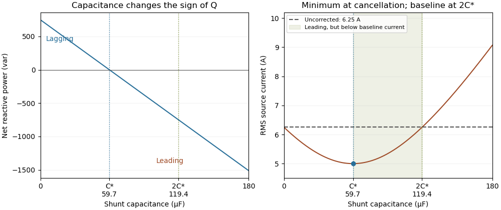
Leading operation begins before correction increases current above the uncorrected value
. Original constant-load model at 200 volts RMS and 50 hertz with 1000 watts active power and 750 vars inductive reactive power. Optimal correction is about 59.68 microfarads. Between 59.68 and 119.37 microfarads the source is leading but still draws less current than the uncorrected load; above 119.37 microfarads it draws more. Details.
The optimum changes with the load. If the example load's and both halve while its original optimal correction remains connected, then and . Source electric current is 3.125 amperes and the factor is 0.8 leading. This dependence motivates automatic power factor correction. The cited controller description measures system electric potential difference and electric current, using external current transformers, and switches discrete capacitor bank stages to follow a target.[ref]
Retain the phase or sign of when reporting the result. A bare power factor magnitude does not distinguish leading from lagging; the manufacturer FAQ also illustrates how a meter's signed display depends on its convention.[ref]
Power factor sign conventions in Schneider Electric FAQ FA212521. Resolution and displayed IEC/IEEE convention diagrams
The calculation assumes sinusoidal steady state; current distortion factor is a separate consideration for nonsinusoidal current.The current reduction interval for shunt reactive compensation is the range of ideal capacitive corrections that draws less source RMS electric current than the uncorrected inductive load. It is wider than the range that avoids reactive power overcompensation.
Assume fixed sinusoidal RMS electric potential difference , active power , and inductive reactive power . Let be the magnitude of the added capacitive reactive power. Comparing squared source electric currents givesConsequentlyor with . The model's capacitive reactive power follows the sinusoidal complex electrical power convention.[ref]
At , source electric current is smallest. Between and , the source has a leading power factor but still draws less electric current than before correction. At , the residual reactive power is : its magnitude matches the original value, restoring the original source-current magnitude. Beyond that point the corrected electric current is larger.
For an original example, choose , and . Uncorrected electric current is . Full cancellation gives . An overcorrection leaves and draws only . But restores , and increases it to .
Two choices and are symmetric around the optimum and give the same squared source electric current. This symmetry explains why power factor magnitude alone cannot identify the sign of the residual reactive power. If , no positive reduces current under the same fixed-load assumptions.
With the same upstream electrical resistance, reducing source mean-square electric current also reduces that conductor's Joule heating. It does not erase the current carried by the local capacitor branch or assess its ratings. Harmonic interactions, nonideal components and changing load conditions need their own model; this interval is an exact statement about the stated one-frequency circuit.
Articles by others on the same topic
There are currently no matching articles.