A capacitor stores electrostatic energy by separating electric charge between two electrical conductors. In the ideal two-terminal model their electric charges are and , with a vacuum or insulating gap preventing direct transfer between them. Write for the terminal electric potential difference, where and are the electric potentials of the two electrical conductors. A linear capacitor obeyswhere its capacitance depends on the geometry and permittivity, and is independent of the applied electric potential difference while these stay fixed. [ref].
For example, the parallel-plate capacitor below has capacitance . At terminal electric potential difference , the electric charge magnitude on either plate isThe total electric charge of the device is : charge neutrality does not imply zero capacitor energy. This capacitor stores in its electric field. The schematic in parallel-plate capacitor shows the separation of electric charge; the plots in capacitor energy show how storage grows with terminal electric potential difference.
The useful distinction is between storing net electric charge and storing separated electric charge. A capacitor can release electrostatic energy into an electrical circuit; in an ideal RLC circuit, energy moves between the capacitor's electric field and the magnetic field associated with inductance. An ideal disconnected capacitor retains its separated electric charges and capacitor energy because there is no path for discharge.
An ideal constant-voltage source charging an initially uncharged capacitor through a series resistor gives and . These follow from Kirchhoff's voltage law and . A smaller time constant means faster fractional settling; it does not fix the initial current or final charge unless the separate values of and are specified.
Feed a node through resistance from an ideal voltage , connect that node to ground through , and connect a capacitor from it to a second node grounded through . The capacitor sees a Thévenin equivalent with open-circuit voltage and resistance . For zero initial capacitor voltage, and . The branch current is , so the two branch currents coincide at . This illustrates why the source-side resistor alone does not determine a charging time constant.
With current entering the positive-voltage terminal, differentiating the capacitor charge relation at fixed capacitance gives . A changing voltage drives current through the external circuit while a changing electric field supplies displacement current across an ideal vacuum gap.
For an ideal linear capacitor, the electric charge on the plate at positive electric potential difference is , where is its capacitance. The opposite plate carries . An initial charge supplies the integration constant in an op amp integrator.
The voltage across an ideal linear capacitor of constant capacitance C is its signed plate charge divided by C. With the passive current convention, .
Integrating the current-voltage relation shows that a finite electric current cannot change capacitor voltage instantaneously. An imposed impulsive current can make it jump. A prescribed instantaneous short-circuit discharge is an idealization of this exceptional fast process, not a counterexample for finite current.
An electrochemical capacitor storing charge through high-area electric double layers, pseudocapacitance, or a combination. Its device energy depends on usable voltage, inactive mass and rate capability as well as electrode capacitance.
Charge-storage response of separated ionic and electronic charge at an electrode-electrolyte interface. The differential capacitance is ; it can vary with electrode potential, ion packing and surface structure.
Capacitor-like differential charge storage produced by sufficiently fast and reversible Faradaic processes over a useful potential interval. A redox-active nanomaterial is not necessarily pseudocapacitive.
A supercapacitor whose principal storage mechanism is non-Faradaic charge separation at electrode–electrolyte interfaces. The two electrode interfaces contribute series capacitances.
A gate, insulating oxide and semiconductor form a capacitor. Applied electric potential difference changes the near-surface distribution of charge carriers.
A parallel-plate capacitor consists of two parallel electrical conductors with overlapping area and separation . If the gap is small compared with both plate widths and is filled by a uniform material of positive permittivity , its capacitance is approximatelyThis neglects the fringing field of a capacitor near the plate edges. The interior electric field points from the plate of positive electric charge to the plate of negative electric charge, and is approximately uniform. [ref].
For a worked vacuum example, stipulate , , and vacuum permittivity . This rounds the value in Fundamental Physical Constants — Complete Listing by National Institute of Standards and Technology and others. Within the approximation,At terminal electric potential difference , the electric field magnitude is , the plate electric charge magnitude is , and the capacitor energy is . These numbers use the stipulated rounded vacuum permittivity; finite plates also have corrections from the fringing field of a capacitor.
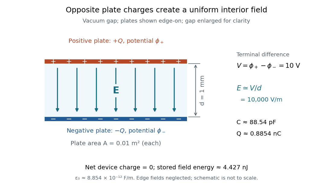
The formula makes design changes easy to predict: doubling the overlapping area doubles the capacitance, and halving the gap doubles the capacitance, with permittivity fixed and the fringing field of a capacitor neglected. Doubling permittivity also doubles capacitance if the material uniformly fills the gap and remains linear. This lets a compact device store more separated electric charge at the same terminal electric potential difference.
The short derivation uses surface charge density . In the interior, Gauss's law gives electric field magnitude . The electric potential difference is , so dividing by gives . A narrow curved capacitor gap has the same leading local approximation when its width is much less than the curvature radius.
For square plates with a linearly varying gap from to , the local-strip approximation gives the displayed capacitance for . Its expansion is . An isolated capacitor has fixed electric charge, so decreases as increases. A sinusoidal small tilt therefore produces a leading energy variation at twice the tilt frequency.
Between large plates at prescribed electric potentials and separation , fixed uniform charge density gives by Poisson's equation. The signed electric field is linear. Its magnitude can have an interior V-shaped minimum, so a sketch of signed field alone need not answer a request for field magnitude.
The fringing field of a capacitor is the nonuniform electric field near the edges of its electrical conductors, extending outside the gap. For a parallel-plate capacitor, neglecting it is useful when the gap is much smaller than both plate widths; the approximation is less reliable when these lengths become comparable.
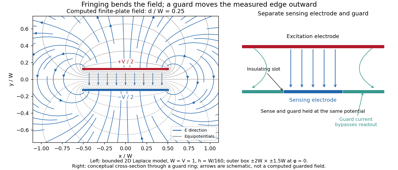
Finite plates break the translational symmetry of the infinite-plate model. Each conductor in electrostatic equilibrium is an equipotential, so the electric field must meet a smooth conducting surface normally. Near an edge, the equipotentials curve into the surrounding space and the electric field changes both direction and magnitude. The surface charge density adjusts to enforce the conducting boundary conditions; it is not uniform all the way to a sharp edge. The electrostatic boundary conditions at a conductor explain why zero electric field inside the metal does not imply zero electric field just outside it.
The practical issue is where the nearly uniform region ends. A probe near the centre can support while a probe close to an edge detects a lateral component and a different magnitude. A total capacitance reading also includes electric flux outside the simple footprint. The fringing field of a capacitor can therefore matter in permittivity measurements even when a central electric field measurement looks nearly ideal. Keysight's three-electrode fixture diverts the fringe contribution away from the measured response.[ref]
Materials Measurement: Dielectric Materials. Solution: fringe capacitance and the three-electrode 16451B fixture
Four uniform square charge-sheet pairs, rotated around a common corner, contribute equal normal fields there. Their superposition is a large central plate pair, so each contributes one quarter of its field. This gives when the bulk charge-voltage relation is used. It is an approximation for prescribed uniform sheets, not an exact equipotential-conductor result. Reflection in the mid-plane does give zero tangential field for either model.
The capacitor gap aspect ratio compares the gap with a lateral plate width . For rectangular plates of widths , require both and for the leading parallel-plate capacitor approximation. Large area alone is insufficient: a long narrow strip can have large area and still have comparable with its smaller width. In addition, the observation point must be many gap widths from an edge. Reducing improves the interior approximation without making the edge itself disappear.
In a two-dimensional straight gap, write the electric potential as the infinite-plate solution plus a perturbation:The perturbation satisfies the Laplace equation and vanishes on the two ideal plates. Separation of variables in a semi-infinite strip, with the distance inward from its entrance, gives transverse modesThus edge disturbances have a natural penetration scale set by . Modes forbidden by a particular symmetry have zero coefficients; this expression is an explanation of localization in an ideal strip, not a universal numerical correction to finite-plate capacitance. The outside boundary conditions determine the coefficients.
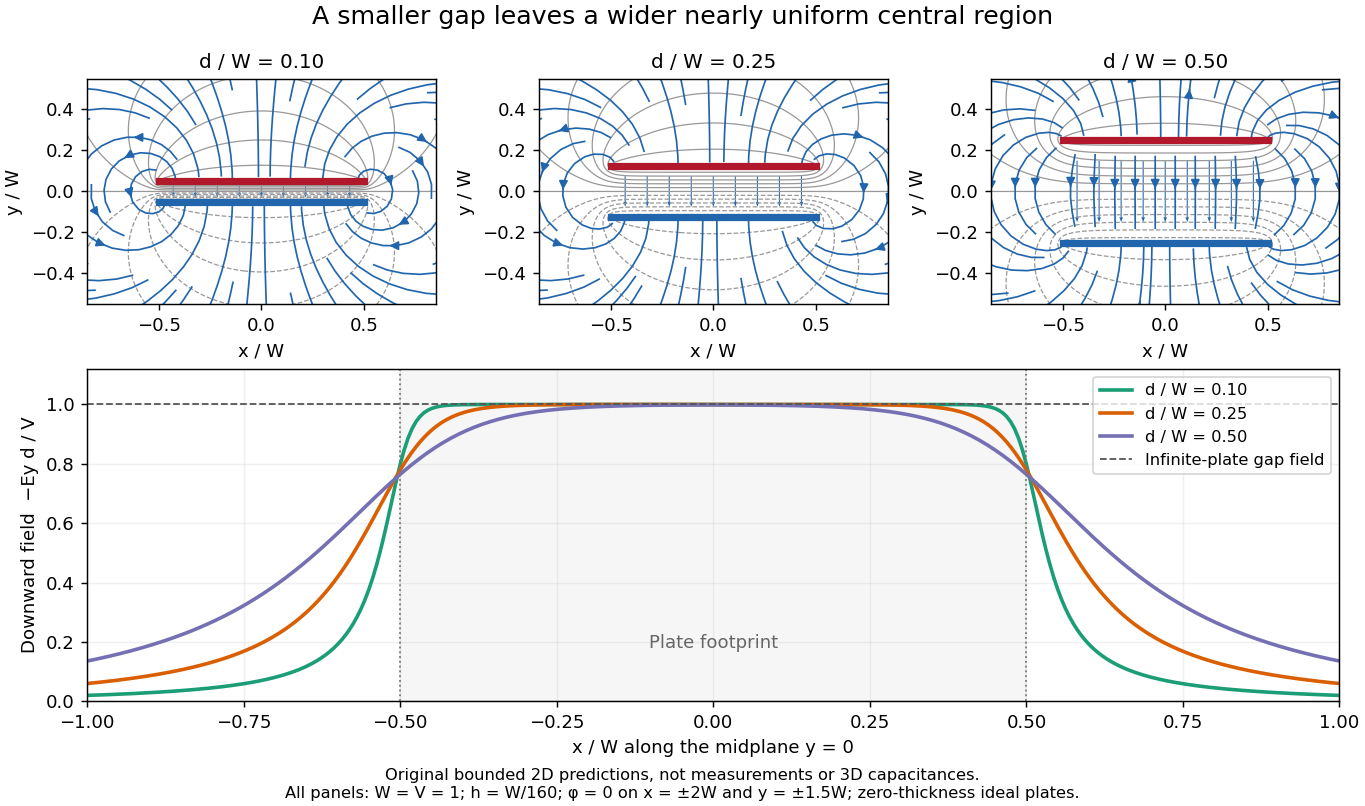
Capacitor gap aspect ratio and the width of the nearly uniform electric field region
. Three original solutions of the same bounded two-dimensional capacitor field model at . The lower curves show on the midplane ; the dashed reference is the infinite-plate value inside the gap. The dashed value is not the infinite-plate prediction outside the plate footprint. All curves are calculated, with the same mesh and outer Dirichlet boundary conditions; they are neither measurements nor an exact open-domain three-dimensional capacitance calculation. Details.There is no single aspect-ratio cutoff guaranteeing an assigned accuracy: the requested observable, plate shape and thickness, surroundings, dielectric distribution, and guard geometry all matter. The small-gap approximation is local and is not uniform across an edge. It also does not justify extrapolating to arbitrarily large , where finite electrical conductors and their external electric field dominate. At fixed , formally shrinking an ideal gap makes the interior electric field grow like ; real electric currents across an imperfectly insulating gap, surface roughness and contact eventually invalidate that ideal limit.
The diagrams solve an explicitly bounded Dirichlet problem in a uniform charge-free medium of constant permittivity. Take a width scale and terminal electric potential difference . Two zero-thickness ideal plate segments occupy at , with electric potentials . Fix on the entire rectangle , . This boundary is an additional enclosing equipotential, rather than a condition at infinity. The model is invariant along the omitted third direction. The connection between the electric potential, its gradient, and the charge-free Laplace equation follows from electrostatics.[ref]
On a square mesh of spacing , the finite difference method imposesat free nodes, while plate and outer nodes retain their prescribed electric potentials. There are nodes. Each plotted gap aligns exactly with the mesh; the smallest gap has 16 mesh intervals. The generators solve the resulting linear system by the Conjugate gradient method, stopping when the maximum dimensionless five-point residual is below , and use central finite differences to approximate away from plate nodes.
The discrete maximum principle keeps the computed electric potential between and . Reflection checks require evenness in and oddness in ; halving tests discretization effects, while enlarging the outer rectangle tests sensitivity to its artificial boundary conditions. These are different checks: a small residual only establishes that the discrete equations were solved. Differentiating near zero-thickness endpoints is especially sensitive to the mesh, so the plots do not report a converged edge peak. No total electric charge, exact open-domain three-dimensional capacitance, or measured material property is extracted from this model.
For a bounded numerical check, compare with the plotted at midplane positions . At , the largest change in is approximately , at ; the other five sampled changes are below . At , moving the outer rectangle from to while retaining changes these samples by at most approximately . These calculated sensitivities support the qualitative comparison and expose its limits; they are not experimental uncertainties or evidence that the artificial boundary has converged to infinity.
The Field Mapper Kit (PK-9023), Product Manual 012-04346D by PASCO scientific (p. 3, Parallel plate capacitor) proposes a direct investigation of the plate-length-to-gap ratio using conductive-paper electric potential mapping. Its finite straight electrodes represent a cross-section of the plates. The apparatus is a gridded resistive sheet on a corkboard, silver-ink electrodes, pushpin electrical contacts, a – direct supply capable of , and a voltmeter with input electrical resistance at least . The manual specifies waiting 20 minutes for the ink to reach its maximum electrical conductivity, then checking each electrode: its internal voltage drop should be no more than of the applied electric potential difference.[ref]
For the readout, keep one voltmeter lead on the reference electrode and scan the other across the sheet. Mark points having the same reading to trace an equipotential. A second method holds the two probe tips at a fixed separation and pivots them to find the largest electric potential difference; a suggested separation is one centimetre. Avoid printed grid marks when making contact.[ref]
Charge, Equipotential, and Field Mapper (ES-9060), Instruction Manual by PASCO scientific. pp. 8–10, Parts III–IV: equipotential tracing and paired-probe field-gradient mapping
The inference follows from the measured electric potential, rather than assuming straight electric field lines. With probe separation and direction , a local finite difference givesAn arrow toward rising electric potential follows , so it must be reversed to show . To investigate the fringing field of a capacitor, compare contours well inside the gap with contours near and beyond the ends, then repeat at a changed gap while keeping the sheet boundary and plate length fixed. Curving contours and an outside gradient establish nonuniformity in this planar setup. Compare at recorded positions to distinguish simple voltage rescaling from geometric changes; no measured values are supplied here.
Additional useful controls are repeat reference readings to detect drift, reversal of supply polarity, and repeating selected readings with reduced probe spacing. Keep contact quality and sheet edges fixed during the aspect-ratio comparison. Finite probe separation averages the gradient; reducing it improves spatial resolution but magnifies the effect of voltage uncertainty. Voltmeter loading, imperfect ink electrodes, and inhomogeneous sheet electrical conductivity can mimic distortions. These proposed checks supplement the manufacturer's electrode check, rather than claiming a completed experiment.
The sheet carries a steady electric current. For uniform electrical conductivity, Ohm's law and electric charge conservation give the two-dimensional Laplace equation away from electrodes, as explained in conductive-paper electric potential mapping. Uncontacted sheet edges have zero normal electric current, whereas the diagram model fixes zero outer electric potential. These distinct boundary conditions must be matched before a quantitative comparison. The apparatus reveals a planar electric potential map; it does not directly measure the free-space three-dimensional capacitance of metal plates.
A guard electrode of a capacitor surrounds an electrically isolated sensing electrode and is held at the same electric potential. The small insulating slot separates their readout paths. The guard extends the nearly planar equipotential, moving the main outer edge away from the sensing region; it does not abolish the fringing field of a capacitor everywhere. In a capacitance fixture, fringe electric current is routed through the guard instead of the sensing readout. Keysight describes this three-electrode method in Materials Measurement: Dielectric Materials (Solution, 16451B fixture).[ref]
Materials Measurement: Dielectric Materials. Solution: guard absorbs current through fringe capacitance
Measuring the sensing and guard electric currents together would include the diverted response again. Grounding an arbitrary surrounding electrode also does not reproduce a guard unless its electric potential matches the sensing electrode. Finite guard width, the insulating slot, plate misalignment and specimen air gaps limit the approximation. Use capacitance measurement calibration and the geometry appropriate to the sensing region when inferring permittivity. The source also warns that guarding changes the electromagnetic field unfavourably at high frequency, so the low-frequency electrostatic picture has a restricted range.[ref]
Materials Measurement: Dielectric Materials. Solution: air gaps, high-frequency guard limitations, fixture compensation
Two concentric conducting spherical shells of radii with charges have an electric field only in the intervening vacuum: by Gauss's law. Integrating gives a potential difference , and hence the displayed capacitance. The electrostatic energy is , either by charging work or by integrating over the gap.
A biased intermediate concentric conductor redistributes the potential drop between two gaps. For radii and boundary voltages , the peak gap fields are and , where and . For positive , moving into cannot increase either field. Within that interval, one field falls and the other rises, so the maximum is minimized at equality. Consequently and . Equal potential drops are generally not optimal.
The capacitor energy is the electrostatic energy stored when electric charge is separated. For a linear capacitor of fixed positive capacitance , plate electric charge magnitude , and terminal electric potential difference , it isThe zero is the uncharged state. Thus the capacitor energy is positive for nonzero , even though the total electric charge of the two plates is zero. [ref].
For the parallel-plate capacitor example, capacitance and terminal electric potential difference giveThe plate electric charge magnitude is . Doubling terminal electric potential difference with capacitance unchanged doubles the plate electric charge magnitude and quadruples the capacitor energy.
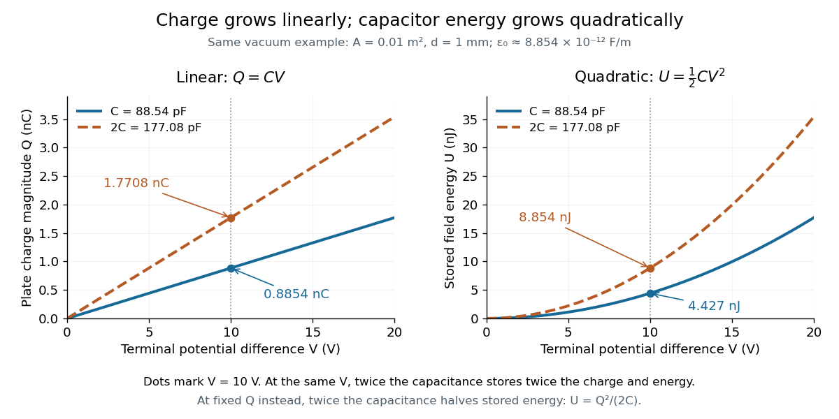
The electric charge is a linear function of terminal electric potential difference, while capacitor energy is a quadratic function. The second curve in each plot uses twice the capacitance: at a given terminal electric potential difference, both plate electric charge magnitude and capacitor energy double. These relations let us calculate how much energy an electrical circuit can receive when a capacitor discharges.
A brief charging argument explains the factor . If the plate electric charge magnitude has reached , the terminal electric potential difference is . Transferring a further amount of electric charge quasistatically requires work . With the geometry and permittivity fixed, the integral isUsing gives the other two forms. This integral accounts for the gradually rising terminal electric potential difference; it is the work stored in the capacitor's electric field, rather than a claim that all energy drawn from a fixed-voltage battery during charging ends up stored.
The field picture gives the same result. In the vacuum gap of a parallel-plate capacitor, the electric field has energy density . Multiplying by the gap volume gives the electrostatic energyFor the worked example, and reproduce . The electrostatic energy resides in the electric field throughout the gap, despite overall charge neutrality.
When capacitance changes, specify the constraint. At fixed plate electric charge magnitude , increasing capacitance decreases capacitor energy ; doubling capacitance halves it. At fixed terminal electric potential difference , increasing capacitance increases capacitor energy ; doubling capacitance doubles it. In the latter case a connected battery supplies additional electric charge and energy, and there may also be mechanical work. Use the fixed-voltage capacitor energy balance to account for all transfers before inferring a force from changing capacitor energy.
For thin parallel circular plates of radius and separation , the quasistatic axial field induces . Integrating cycle-averaged vacuum energy densities for sinusoidal drive gives . The same fields have radial Poynting flux , whose leading net inward power equals the time derivative of stored electric energy. The small ratio diagnoses the quasistatic regime.
For a quasistatic change of capacitance at fixed terminal electric potential difference, the capacitor energy is and plate electric charge is . Electrical work supplied to the electric field by the battery is , so mechanical work done on the capacitor is . Increasing the separation of a parallel-plate capacitor makes : mechanical work is positive even though electrostatic energy decreases, because electrical energy returns to the source. Conversely, when , the battery supplies : half increases capacitor energy and half is available as mechanical work done by the electric field. Differentiating capacitor energy alone at fixed terminal electric potential difference omits this exchange with the battery.
At fixed electric potential difference , a change of capacitance has electrical work input and field-energy increase . The remaining half is mechanical work done by the field, so the force in the direction of increasing overlap is . Equivalently the effective mechanical potential is . For a partially filled coaxial capacitor, this gives , directed inward when . The fringing field of a capacitor supplies the local field gradient and transmits this force even when its small correction to total capacitance is neglected.
Articles by others on the same topic

They can only absorb electrons up to a certain point, but then the pushback becomes too strong, and current stops.
Therefore, they cannot conduct direct current long term.
For alternating current however, things are different, because in alternating current, electrons are just jiggling back and forward a little bit around a center point. So you can send alternating current power across a capacitor.
The key equation that relates Voltage to electric current in the capacitor is:So if a voltage Heavyside step function is applied what happens is:More realistically, one may consider the behavior or the series RC circuit to see what happens without infinities when a capacitor is involved as in the step response of the series RC circuit.
- the capacitor fills up instantly with an infinite current
- the current then stops instantly


Capacitors Explained by The Engineering Mindset
. Source. 2019.