AC power describes energy transfer associated with time-varying electric potential difference and electric current, including the distinction between instantaneous transfer and its average. With the passive sign convention, current enters the terminal marked positive, and instantaneous power absorbed by the element is . A positive value means energy entering the element; a negative value means energy returning through that terminal pair.
For sinusoidal steady operation, choosewhere and are root mean square magnitudes. The cosine-product identity givesAveraging over a complete period removes the second term, giving active power . This derivation separates the energy-transfer average from a twice-frequency oscillation.[ref]
University Physics Volume 2 by Samuel J. Ling and others. §15.4, equations15.12–15.13, sinusoidal average power and RMS quantities
For an original example, , and give active power480W. The oscillating term has amplitude600W, so instantaneous power ranges from−120 to1080W. Over ten complete cycles at50Hz, the net energy absorbed is . Temporary negative power can accompany positive net transfer when an element stores and returns energy.
The product in volt-amperes is the apparent power. In the single-frequency sinusoidal convention, reactive power is , giving360 in reactive volt-amperes for a lagging current with . Complex electrical power packages and , while the power factor distinguishes net transfer from the terminal magnitude product. The primary MIT treatment derives these quantities and makes the peak-versus-RMS convention explicit.[ref]
AC Power Flow in Linear Networks by James L. Kirtley Jr.. Energy and Power, equations61–63; §7.1 RMS Amplitude
A measurement must retain the relative phase of the two channels. Multiplying separately measured RMS magnitudes gives apparent power, not generally active power. For nonsinusoidal signals, the time average of remains the definition of active power, but one phase angle need not describe every harmonic contribution.
The harmonic active power sum expresses average electrical power as the sum of contributions from matching components of periodic terminal electric potential difference and electric current. With a common fundamental frequency and root mean square magnitudes for nonzero harmonic components, writeHere are the signed DC components. The passive sign convention makes the average product absorbed active power. Averaging over a complete fundamental period givesFor finite sums this follows from the cosine-product identity: products of different integer harmonic components average to zero, and matching components give half the cosine of their relative phase. For square-integrable periodic waveforms, the corresponding Fourier series identity follows by continuity of the inner product in the mean-square norm. The orthogonality is a property of the averaging interval and basis, not an assumption that the physical sources are independent.
For an original example, set , , , , and fundamental relative phase . Add third-harmonic magnitudes , with relative phase . ThenThe third-harmonic contribution is , even though the total absorbed active power is positive. The root mean square values satisfy and , so apparent power is about and total power factor about .
For a purely sinusoidal supply with no DC component, only survives, giving even if the electric current is distorted. Current in other harmonic components can still increase conductor heating. The usual one-frequency complex electrical power construction is derived in the primary MIT treatment; the sum above applies that average-product reasoning separately to orthogonal components.[ref]
AC Power Flow in Linear Networks by James L. Kirtley Jr.. Energy and Power, equations 45–63; §7.1, RMS amplitudes
A proposed measurement records the two waveforms synchronously and compares their directly averaged product with the resolved sum. A non-integer-period window, unresolved harmonic components, channel timing error or changing waveform can spoil the simple finite-record equality. The formula assumes a shared periodic model; multiplying separately measured RMS magnitudes gives apparent power instead.
The power factor is the ratio of active power to the product of RMS terminal electric potential difference and electric current:when the denominator is positive. It measures how effectively those terminal magnitudes support net average transfer. With signed absorbed power it can be negative for net generation; for an absorbing load the usual range is zero to one. The Cauchy-Schwarz inequality applied to the time average of proves .
For one-frequency sinusoids, , so the power factor is . The phase-only quantity for the fundamental is also called displacement power factor. The primary treatments make the RMS convention explicit.[ref]
University Physics Volume 2 by Samuel J. Ling and others. §15.4, equations15.12–15.13
[ref]AC Power Flow in Linear Networks by James L. Kirtley Jr.. Energy and Power, equation62; §7.1 RMS Amplitude
A distorted current can give another result. For purely sinusoidal supply potential difference and a zero-mean current with fundamental RMS magnitude ,Only the in-phase fundamental contributes to the average product with that supply waveform. For an original example with fundamental3A in phase and third-harmonic RMS magnitude4A, total RMS current is5A. The displacement power factor is one but total power factor is0.6. Changing the fundamental phase alone would not remove this harmonic-current contribution.
At fixed absorbed active power and supply RMS potential difference, . For an original900W,230V example, changing the factor from0.6 to0.9 changes source current from about6.52 to4.35A. In the same upstream resistance, the corresponding loss becomes of its former value. This is a stipulated circuit calculation, not an assertion about a particular tariff or installation.
Power factor correction addresses the mechanism causing the low ratio. An ideal capacitive branch can offset inductive reactive power at one frequency; it does not automatically correct an arbitrary distorted current. State the waveform conditions and whether the reported number is total or displacement factor when comparing measurements.
A lagging power factor describes an absorbing sinusoidal electrical load whose electric current lags its terminal electric potential difference. With the passive sign convention, chooseThe current maximum occurs later by . The RMS phasors give complex electrical powerIn this equation the supply phasor is the real number , while denotes the conjugate of the current phasor. Positive is inductive reactive power under this convention. The primary MIT notes derive the conjugation and the peak-versus-RMS factor.[ref]
For an original , example with , active power is and reactive power is . At , radians corresponds to a current delay of about . The factor gives the magnitude of the phase relationship, while the word lagging supplies the direction lost by the cosine.
An ideal inductor is the limiting case : it alternately stores and returns magnetic energy, with zero mean active power. An absorbing resistive-inductive load usually has both positive active power and positive reactive power. An ideal parallel capacitor can reduce the source's quadrature electric current; sufficient extra capacitance eventually crosses into leading power factor rather than improving the factor indefinitely.
For distorted waveforms, specify whether lagging refers to the fundamental displacement power factor; one phase angle does not characterize arbitrary harmonic components. A signed meter display is also not a universal lead/lag label. The manufacturer's sign-convention explanation distinguishes phase direction from the convention used for displayed factor signs.[ref]
Power factor sign conventions in Schneider Electric FAQ FA212521. Resolution, lead/lag description and IEC/IEEE display-convention diagrams
A leading power factor describes an absorbing sinusoidal electrical load whose electric current leads its terminal electric potential difference. Under the passive sign convention, writeThe current maximum occurs earlier by . The complex electrical power isThe negative reactive power is consistent with a capacitive terminal response. It does not imply negative mean absorbed active power.
For an original , example with , the power factor magnitude is , active power is , and reactive power is . At the current leads by . A load with the same RMS magnitudes and the opposite phase displacement has identical active power but a lagging power factor and opposite reactive power.
For an ideal capacitor, gives a quarter-cycle current lead. Its mean active power is zero, although instantaneous power alternates as electrical energy enters and leaves the field. The primary one-frequency power derivation separates this quadrature exchange from net energy transfer.[ref]
An inductive load can acquire a leading power factor at the source when power factor correction supplies more capacitive reactive power than the load absorbs. The current reduction interval for shunt reactive compensation shows why mildly leading operation can still draw less source electric current than no correction, while excessive correction reverses that benefit.
Record phase direction or signed reactive power together with the numerical factor. The same positive cosine can describe leading and lagging loads, and a meter may assign a separate sign according to its display convention.[ref]
Power factor sign conventions in Schneider Electric FAQ FA212521. Resolution and IEC/IEEE convention diagrams
For nonsinusoidal signals, state whether leading describes the fundamental displacement power factor; the complete power factor also depends on waveform distortion.The current distortion factor is the ratio , where is the root mean square magnitude of the fundamental electric current component and is the root mean square magnitude of the complete electric current. Its square is the fraction of the current's mean square supplied by the fundamental component. This ratio is distinct from displacement power factor, which measures the relative phase of the fundamental potential difference and current.
Use a Fourier series at fundamental frequency :Here is the DC component and the are RMS magnitudes of harmonic components. Averaging over a complete period, orthogonality and the Parseval identity giveFor purely sinusoidal electric potential difference , only the fundamental electric current contributes to active power:Thus a displacement power factor of one can coexist with a lower total power factor.
For , use fundamental-normalized current total harmonic distortion, . The relation between current distortion factor and THD with DC current isWith zero DC component, this reduces to . The definition of RMS here includes the DC component. For example, a 10 ampere fundamental and 3 ampere DC component, with no higher harmonic components, have zero total harmonic distortion but .
For an original zero-mean waveform, take a 230 volt RMS sinusoidal supply, , , and RMS third/fifth harmonic components of 6 and 3 amperes. ThenThe active power is 1840 watts, apparent power is about 2769.57 volt-amperes and total power factor is about 0.6644. This is an illustrative waveform model, not a measurement of a particular rectifier.
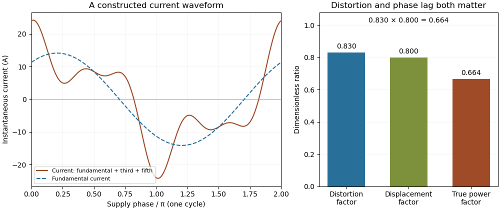

Terminology requires care. Overview of Functions: Harmonic Measurements by Schneider Electric uses distortion factor for the ratio of power factor to the fundamental cosine. Power Quality Considerations by Schneider Electric uses the label for harmonic content relative to the fundamental, or total harmonic distortion. The defining ratio identifies the intended quantity.
If the supply also contains harmonic components, use the harmonic active power sum:with matching voltage/current phase conventions. The fundamental-only factorization above assumes a purely sinusoidal supply.
The relation between current distortion factor and THD with DC current accounts for the mean component omitted from the usual fundamental-normalized total harmonic distortion. For a periodic electric current, let be its signed DC component, the fundamental RMS magnitude, and the RMS magnitudes of higher harmonic components. The Parseval identity givesDefine and current distortion factor . Division by provesThe root mean square in this expression includes the mean, while the stated total harmonic distortion excludes it. An instrument reporting AC-only RMS or a differently normalized distortion quantity requires a correspondingly different conversion.
For an original example, take , and combined higher-harmonic RMS magnitude . Then , and . Neglecting the DC component would instead predict . In the same conductor electrical resistance , the actual heating is , while that omission would predict .
For a zero-mean sinusoidal supply of RMS and an in-phase fundamental current, the example absorbs . Its apparent power is approximately , so total power factor is despite a displacement power factor of one. The DC component carries no average power from that particular zero-mean supply, but it still increases mean-square electric current. If the supply itself has a DC component, its contribution must be included through the harmonic active power sum.
As tends to zero the defining current distortion factor can tend to zero, but fundamental-normalized total harmonic distortion is undefined at . Do not evaluate the boxed relation there by silently dividing by zero. The manufacturer's documentation also uses differing labels for distortion ratios, reinforcing the need to state the defining normalization.[ref][ref]
Overview of Functions: Harmonic Measurements by Schneider Electric. Quality Indicators, Distortion Factor
Power factor correction changes the current drawn from a source so that a specified active power is supplied with a more favorable power factor. For a sinusoidal inductive load, a parallel capacitor can supply an opposite reactive power component. It changes the source current's quadrature component while an ideal lossless correction branch leaves the load's active power unchanged.
Let the original load absorb at RMS potential difference and angular frequency . A parallel ideal capacitance contributes , soTo change a lagging phase angle from to a smaller lagging angle at fixed ,These follow from complex electrical power and the capacitive phase relationship.[ref]
AC Power Flow in Linear Networks by James L. Kirtley Jr.. Energy and Power, equations61–65; capacitive/inductive terms in equation71
For an original ideal example, take , and50Hz. An initial factor0.8 corresponds to750var. A target factor0.95 corresponds to about328.68var, so a capacitance about33.53µF supplies the difference. RMS source current changes from6.25A to about5.26A. Resistive feeder loss at fixed resistance changes by , while the1000W load conversion remains the same in this model.
Reactive power overcompensation occurs if the capacitive contribution exceeds the intended inductive component. The net then changes sign; continuing to add capacitance does not keep improving the magnitude of the factor. At a different load or frequency the same component can produce another result. Component ratings and nonideal circuit behavior require their own model rather than being determined by this one-frequency algebra.
Correction of displacement power factor is also distinct from correction of waveform distortion. Harmonic current can remain after the fundamental quadrature component is canceled. A useful measurement compares synchronized source potential-difference/current waveforms, RMS magnitudes and their average product before and after a change, retaining the operating condition. Separately measuring only RMS magnitudes cannot establish the resulting active power.
Automatic power factor correction adjusts a correction device as the measured load changes, rather than leaving one fixed compensating setting connected. In a staged capacitor bank, a controller uses terminal electric potential difference and electric current information to choose which stages are connected. The controlled quantity and target must distinguish active power, signed reactive power, waveform distortion and the chosen lead/lag convention.
For an original single-phase sinusoidal model, available stages each supply of capacitive reactive power at the operating electric potential difference. With connected stages,At fixed , maximizing the magnitude of the power factor chooses the available integer minimizing . Away from the end limits, nearest-stage rounding leaves . This capacitor-stage quantization error can be positive or negative. A policy forbidding leading operation instead restricts , so it can choose a different setting.
Suppose , and . Three stages leave and factor about leading; two stages leave and factor about lagging. Both outcomes are consistent with their respective objectives. If the load changes to , , leaving all three stages connected produces ; zero stages is closer to cancellation than one. A stored stage decision must therefore be updated when the load changes.
Actual feedback must measure the corrected network. The Eaton paper places the current transformer so it senses the relevant load and capacitor contribution, and explains how a wrong phase, polarity or location produces misleading feedback.[ref]
Capacitor Application Issues by Thomas M. Blooming and Daniel J. Carnovale. Section VI.C, printed p.8, CT Location for Automatic Banks
Measuring only the correction branch would not establish the combined source power factor.A proposed controller test varies a known resistive-inductive load through several operating points, recording stage state, signed reactive power, RMS electric current and synchronized terminal waveforms. Check both increasing and decreasing demand, including small excursions around a stage threshold. A dead band and timing rules can prevent repeated switching in response to small fluctuations; they must be specified along with the target. Stage size, switching transients and the load's harmonic components require additional checks beyond the ideal rounding model.
Capacitor-stage quantization error is the residual reactive power caused by choosing among discrete settings of a capacitor bank instead of a continuously adjustable correction. In a fixed sinusoidal operating model, let the load absorb and let the target residual be . The desired capacitive correction is . Selecting available correction leavesThe error concerns the selected setting, separately from sensing error, changing load and component tolerance.
For equal stages of magnitude and an available range covering the desired correction, nearest-stage selection chooses an integer nearest . HenceAt a half-stage tie either neighbor attains the bound. A policy forbidding a negative residual relative to zero instead rounds downward and gives , away from the bank's capacity limits. The two policies solve different constrained problems.
For an original zero-target example, let and . Three stages give ; two give . With active power , nearest-stage selection guaranteesprovided the zero-reactive target is within range and the sinusoidal fixed-load assumptions hold. At only , the same worst-case bound falls to about . A stage size suitable at high demand need not give the same numerical power factor at low demand.
Unequal stages require the actual attainable set. Stages of 100 and 400 vars permit vars. At a desired 250 vars, the nearest setting leaves 150 vars error, despite the smallest stage being only 100 vars. The relevant bound is half the largest gap between neighboring attainable settings in the tested range, not half the smallest component. Outside the bank's range, clipping to an endpoint can leave a larger error.
At fixed frequency, a fixed capacitance gives , so stage magnitudes also change with RMS electric potential difference. Eaton's paper describes discrete stage sizes, combinations and automatic control; the error bounds above are original consequences of that ideal setting model.[ref]
Capacitor Application Issues by Thomas M. Blooming and Daniel J. Carnovale. Section V.C–D, printed p.6, stage sizes and fixed versus switched capacitors
A proposed test records the actual stage states and terminal quantities while slowly varying a known load across thresholds. Compare the observed residual with the attainable-setting prediction before assigning every deviation to quantization.Optimal shunt capacitance for sinusoidal power factor correction minimizes the source's RMS electric current for an ideal fixed sinusoidal supply and a fixed load with active power and inductive reactive power . A lossless parallel capacitor supplies signed reactive power , where is the supply RMS electric potential difference and the angular frequency.
The squared source electric current isDifferentiating givesThus the unique minimum isThe fundamental quadrature electric current vanishes there. Strict convexity proves this is a global optimum in the stated model, rather than merely a stationary point. The capacitive sign and one-frequency complex electrical power relation follow from the primary MIT derivation.[ref]
AC Power Flow in Linear Networks by James L. Kirtley Jr.. Energy and Power, equations 61–65 and 71; §7.1 RMS amplitudes
For an original example, , , and give . Source electric current falls from to . A capacitance 20% below or above leaves or , respectively, and both draw about . They have the same power factor magnitude, about , but opposite lead/lag direction.
The exact excess above the optimal squared electric current isSmall sizing errors therefore affect this loss objective quadratically around the optimum, while residual reactive power changes linearly and changes sign. An allowed interval clips the optimum to its nearest feasible point. If the original load has , the constrained optimum for added nonnegative capacitance is instead .
The result assumes a fixed load, ideal sinusoidal supply, lossless correction and no additional network effects. It does not optimize a system with waveform distortion, component heating, variable terminal electric potential difference or discrete stages. The current reduction interval for shunt reactive compensation describes a wider set of beneficial choices, while automatic power factor correction follows a changing load with available stages.
Reactive power overcompensation occurs when capacitive correction exceeds the inductive reactive power that it is intended to cancel. Under the passive sign convention and a positive-frequency sinusoidal supply, the source then sees negative net reactive power, producing a leading power factor. This can happen when a fixed capacitor bank remains connected as the inductive load falls. Eaton's application paper discusses excessive leading operation and the use of switched correction stages.[ref]
Capacitor Application Issues by Thomas M. Blooming and Daniel J. Carnovale. SectionV, printed p6, switched-bank control and overcompensation
Consider an ideal fixed RMS electric potential difference at angular frequency , supplying a load that absorbs constant and . Let be the magnitude of the correction's reactive power; its signed contribution is . Adding ideal shunt capacitance givesThe model holds the load and supply fixed while changing . It omits losses and additional network dynamics. Optimal shunt capacitance for sinusoidal power factor correction follows by minimizing the squared root mean square electric current:For the remaining reactive power is positive and the power factor is lagging. For it is negative and the power factor is leading. The overcompensation threshold is , but the current reduction interval for shunt reactive compensation is wider. Comparing the square of the corrected and uncorrected electric current givesThus source RMS current is reduced for , equals the uncorrected value at , and is larger for . An overcompensated operating point between and still draws less source electric current than the uncorrected load.
For an original example, keep the parent article's chosen , , and 50 hertz. The uncorrected source draws 6.25 amperes at power factor0.8. Full cancellation needs and reduces source electric current to 5 amperes. A 100 microfarad correction gives and 5.605 amperes, with a leading factor about0.8920. A 150 microfarad correction instead gives about and7.563 amperes, worse than no correction. The crossing is .
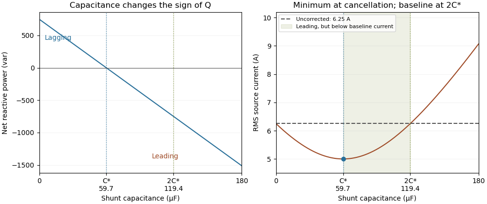
Leading operation begins before correction increases current above the uncorrected value
. Original constant-load model at 200 volts RMS and 50 hertz with 1000 watts active power and 750 vars inductive reactive power. Optimal correction is about 59.68 microfarads. Between 59.68 and 119.37 microfarads the source is leading but still draws less current than the uncorrected load; above 119.37 microfarads it draws more. Details.
The optimum changes with the load. If the example load's and both halve while its original optimal correction remains connected, then and . Source electric current is 3.125 amperes and the factor is 0.8 leading. This dependence motivates automatic power factor correction. The cited controller description measures system electric potential difference and electric current, using external current transformers, and switches discrete capacitor bank stages to follow a target.[ref]
Retain the phase or sign of when reporting the result. A bare power factor magnitude does not distinguish leading from lagging; the manufacturer FAQ also illustrates how a meter's signed display depends on its convention.[ref]
Power factor sign conventions in Schneider Electric FAQ FA212521. Resolution and displayed IEC/IEEE convention diagrams
The calculation assumes sinusoidal steady state; current distortion factor is a separate consideration for nonsinusoidal current.The current reduction interval for shunt reactive compensation is the range of ideal capacitive corrections that draws less source RMS electric current than the uncorrected inductive load. It is wider than the range that avoids reactive power overcompensation.
Assume fixed sinusoidal RMS electric potential difference , active power , and inductive reactive power . Let be the magnitude of the added capacitive reactive power. Comparing squared source electric currents givesConsequentlyor with . The model's capacitive reactive power follows the sinusoidal complex electrical power convention.[ref]
At , source electric current is smallest. Between and , the source has a leading power factor but still draws less electric current than before correction. At , the residual reactive power is : its magnitude matches the original value, restoring the original source-current magnitude. Beyond that point the corrected electric current is larger.
For an original example, choose , and . Uncorrected electric current is . Full cancellation gives . An overcorrection leaves and draws only . But restores , and increases it to .
Two choices and are symmetric around the optimum and give the same squared source electric current. This symmetry explains why power factor magnitude alone cannot identify the sign of the residual reactive power. If , no positive reduces current under the same fixed-load assumptions.
With the same upstream electrical resistance, reducing source mean-square electric current also reduces that conductor's Joule heating. It does not erase the current carried by the local capacitor branch or assess its ratings. Harmonic interactions, nonideal components and changing load conditions need their own model; this interval is an exact statement about the stated one-frequency circuit.
The displacement power factor is , where is the phase difference between the fundamental components of terminal electric potential difference and electric current. It describes phase displacement at that frequency. For purely sinusoidal signals it equals total power factor; with distorted waveforms those quantities can differ. The one-frequency phase relation follows from the RMS average-power expression.[ref]
University Physics Volume 2 by Samuel J. Ling and others. §15.4, equations15.12–15.13
For a purely sinusoidal potential difference of RMS magnitude and zero-mean periodic current, orthogonality of harmonics givesThe ratio is the current distortion factor under these assumptions. A displacement factor near one does not establish that the whole current waveform closely follows the supply sinusoid.
For an original example, let the supply be100V RMS. Let the fundamental current be4A RMS at a lagging phase with cosine0.8, and add a3A RMS third harmonic. Total RMS current is5A, active power320W and apparent power500VA. The displacement factor is0.8 while total power factor is0.64.
Now cancel only the fundamental quadrature current, whose magnitude is . The remaining in-phase fundamental is3.2A and the third harmonic is still3A. RMS source current is , so total factor is about0.73 even though the displacement factor has become one. This illustrates a limitation of phase-only power factor correction, not a universal model of a correcting device.
The cosine also loses lead/lag sign: phases and have the same displacement factor but opposite sinusoidal reactive power. Retain the phase or lead/lag convention when that distinction matters. If the potential difference itself contains harmonics, total active power needs the contributions of the corresponding harmonic pairs; this simple fundamental-only reduction is no longer sufficient.
Complex electrical power represents the active and reactive parts of sinusoidal electrical energy transfer in one complex number. Using phasors and whose magnitudes are root mean square values, with the passive sign convention, defineThe star denotes a complex conjugate. The real part is active power; the imaginary part is reactive power. The magnitude is apparent power. A source using peak-amplitude phasors instead has the factor : .[ref]
AC Power Flow in Linear Networks by James L. Kirtley Jr.. Equation63 and §7.1, explicit amplitude convention
To see why the conjugate matters, write and . Then depends on the relative phase. Changing the common time reference multiplies both phasors by , leaving unchanged. The product would instead acquire and would not represent a time-reference-independent average-power quantity.
For an original example, choose and . ThenThus active power is400W, reactive power is300 reactive volt-amperes and power factor is0.8. The corresponding electrical impedance is . With RMS current magnitude5A, the resistive term absorbs , agreeing with the real part.
Under the stated sign convention and time convention, an inductive reactance gives positive and a capacitive reactance negative . Negative does not mean a negative dissipated-energy average. For example, adding an ideal parallel capacitive branch contributing cancels this example's reactive part, leaving terminal complex power400VA and RMS source current4A at100V, while the original resistive dissipation stays400W.
This one-frequency representation must not be applied indiscriminately to a distorted waveform. Different harmonics need their own phase relationships; the definition of active power remains the time average of the actual instantaneous power.
Apparent power is the product of RMS terminal electric potential difference and electric current, conventionally expressed in volt-amperes:For sinusoidal signals at one frequency, it equals the magnitude of complex electrical power and satisfies . It is not generally the average rate of net energy absorption, which is active power.[ref]
AC Power Flow in Linear Networks by James L. Kirtley Jr.. Energy and Power, equations61–63 and §7.1, apparent/complex power and RMS convention
For an original example, a100V terminal pair carrying5A RMS has500VA of apparent power. If active power is400W, the power factor is0.8. In the sinusoidal case the magnitude of reactive power is reactive volt-amperes; the magnitude calculation alone does not determine whether the current leads or lags.
Magnitudes do not add like complex quantities. Consider two parallel sinusoidal loads at the same supply, with complex powers and in volt-amperes. Each has500VA of apparent power, but the combined terminal complex power is600VA with zero imaginary part. The source therefore sees600VA rather than the1000VA sum of individual magnitudes. Their internal branch currents and individual component requirements still exist; reactive cancellation at the source does not erase those branch conditions.
For nonsinusoidal waveforms, the product definition remains useful, but the simple equality with the magnitude of one fundamental-frequency complex power needs qualification. With and , RMS current is5A and apparent power is500VA. The fundamental-frequency complex electrical power is only300VA. The extra RMS current is not represented by that one complex number.
Thus record the waveform convention with an apparent power rating or measurement. Separately measuring RMS potential difference and current gives this product, while recovering active power requires the corresponding average product or adequate phase-resolved information. The Cauchy-Schwarz inequality guarantees without assuming a sinusoidal waveform.
The volt-ampere, symbolVA, is the unit commonly used to express apparent power. At a terminal pair, RMS potential difference in volts multiplied by RMS current in amperes gives the numerical value in volt-amperes. The unit product has the same coherent SI dimensions as the watt:This unit identity does not make apparent power and active power the same quantity. The SI text explicitly warns that different physical quantities can share a unit and that the quantity must be specified.[ref]
The International System of Units (SI), ninth edition, SI Brochure. NIST SP330 parallel text, §2.3.4, coherent derived units and quantity identification
For an original example,250V RMS at8A RMS gives2000VA, or2kVA. If the absorbing load has power factor0.75, its active power is1500W. A1500W value cannot be inferred from the2kVA alone without the phase/waveform information summarized by that factor.
Hypothetical equipment can have separate apparent- and active-power limits. A1000VA/600W limit would permit a500W, factor0.5 load only at the apparent-power boundary, since it requires1000VA. A700W, factor-one load would require only700VA but exceed the separate600W limit. These examples interpret stated numerical constraints rather than specify an actual product's behavior.
For single-frequency sinusoids, the magnitude of complex electrical power is expressed in volt-amperes, while its real part is commonly expressed in watts and its imaginary part in reactive volt-amperes. Those names help keep the quantities distinct even though their base-unit dimensions agree.[ref]
AC Power Flow in Linear Networks by James L. Kirtley Jr.. Energy and Power, equations61–63; §7.1 RMS Amplitude
With distorted signals, retain the actual RMS-product definition of apparent power rather than assuming a single fundamental phasor accounts for all current.Reactive power is the imaginary part of complex electrical power in sinusoidal steady operation. With RMS phasors, the passive sign convention and time convention,where is potential-difference phase minus current phase. Inductive current lag gives positive , while capacitive current lead gives negative . Its conventional unit is the reactive volt-ampere, written var. These definitions retain the specified phasor and sign conventions.[ref]
AC Power Flow in Linear Networks by James L. Kirtley Jr.. Energy and Power, equations61–65; §7.1, RMS amplitudes
The physical role is periodic energy exchange rather than an additional dissipated-energy average. For an ideal inductor, and stored energy is , so . Its energy returns to its initial value after a steady cycle and mean absorbed power is zero. Nevertheless,For an ideal capacitor, , with the negative sign representing the opposite exchange phase. Primary circuit derivations explicitly separate these exchanges from resistor dissipation.[ref]
University Physics Volume 2 by Samuel J. Ling and others. §15.4, Figure15.16, ideal inductive/capacitive instantaneous power
For an original example, , and give . Peak stored energy is0.50J and mean stored energy0.25J, consistent with . Zero ideal average dissipation therefore does not mean zero current or zero energy storage.
For a separate ideal single-frequency compensation example, a100V load with can have its source reactive component canceled by a parallel capacitor satisfyingThe capacitor contributes , leaving400W of source active power and4A RMS source current. This illustrates power factor correction under the stated ideal assumptions, rather than selecting a real component or proving its ratings.
Reactive exchange can increase the current carried through resistive wiring and thereby affect real losses. For distorted waveforms, definitions of non-active power need additional care; the one-frequency imaginary-part definition should not silently be extended to every waveform.
The reactive volt-ampere, conventionally called the var and written with symbolvar, expresses reactive power. The official SI text notes the IEC's special name and states that its coherent unit is identical to the volt ampere. The name identifies the reactive quantity; it is not a different base-unit dimension.[ref]
The International System of Units (SI), ninth edition, SI Brochure. NIST SP330 parallel text, §2.3.4, paragraph identifying the IEC var
In sinusoidal steady operation with RMS magnitudes and relative phase ,Thus100V RMS,2A RMS and a lagging phase with give120var. Under the same passive and phasor conventions, a leading phase of equal magnitude gives−120var. The signed value describes exchange phase rather than negative dissipated heating. The prefix relation is .
A reactive-power value is also not an amount of stored energy in joules. For an ideal inductor in sinusoidal steady operation,For an original200var example at50Hz, mean stored energy is and peak stored energy is twice that. The average absorbed active power is nevertheless zero in the ideal inductor. The primary circuit treatment derives this separation between energy storage and mean dissipation.[ref]
In a sinusoidal100V example with , the reactive component is300var, the active component400W and apparent power500VA. Adding400 and300 as ordinary scalar powers would not give the500VA magnitude. Complex electrical power retains the phase relation needed for this combination.
Active power, also called real power, is the time average of instantaneous power transferred through a terminal pair. For periodic electric potential difference and electric current of common period , the passive sign convention givesThe net energy entering during each period is . Positive active power denotes net absorption under this convention; it can represent useful conversion to other forms of energy as well as heating.
For sinusoids of RMS magnitudes and with relative phase , . For a pure resistor with constant resistance , the stronger waveform-independent statement follows from :This is why the root mean square current is the constant-current value giving the same heating in that resistor.[ref]
An original harmonic example shows why RMS values alone do not determine active power. Letin volts and amperes. Orthogonality over a period gives , but the third harmonic averages to zero when multiplied by the fundamental potential difference. Consequently , whereas apparent power is . The power factor is0.6 even though the fundamental current is exactly in phase with the fundamental potential difference.
More generally, Fourier analysis of real periodic waveforms with RMS harmonic magnitudes giveswhen the expansion and average are justified. Cross terms of different harmonic orders vanish. A single fundamental-frequency complex electrical power therefore need not capture every harmonic contribution to the total average.
For an ideal inductor or capacitor in periodic steady operation, the stored energy returns to its starting value each cycle, so its net active power is zero despite nonzero exchange during the cycle. Real components can also have losses. The primary MIT treatment explicitly separates resistor dissipation from periodic inductive and capacitive energy exchange.[ref]
Articles by others on the same topic
There are currently no matching articles.