RNA melting hysteresis is dependence of an RNA optical melting trace on thermal history: heating and cooling can give different absorbance at the same temperature. It warns that the observed trace may not follow reversible chemical equilibrium on the measurement timescale. Two different traces do not by themselves establish two equilibrium melting temperatures.
A primary experiment illustrates the importance of history. A 21-nucleotide RNA showed a low-temperature dimer-to-hairpin transition that did not reverse on cooling, whereas its higher-temperature RNA hairpin melting transition was reversible. Measurements used a Cary 100 spectrophotometer, a 1-cm quartz cell and 268-nm light, heating at and cooling at or . An adjacent solvent cell held the temperature probe.[ref]
Conversion of stable RNA hairpin to a metastable dimer in frozen solution by Xueguang Sun and others. Results, Fig.5 and transition reversibility; Materials and Methods, UV absorbance melting curves.
The authors interpreted the dimer as kinetically trapped under those conditions, rather than applying a reversible equilibrium fit to that transition.For an original simple kinetic model, let be the unfolded fraction, its equilibrium value and an RNA melting relaxation time:After a fixed-temperature step with constant , the deviation undergoes exponential decay:With stipulated , and , the fraction reaches only 0.632 after two minutes and 0.950 after six. During a continuing temperature ramp, this lag can put heating and cooling on different branches. This single-time model is illustrative; it is not a fit to the published dimer experiment.
Useful checks compare ramp speeds and include fixed-temperature holds and repeat cycles. Verify measurement calibration and exclude evaporation or chemical degradation before attributing a discrepancy to folding kinetics. Slower scans can reduce kinetic lag, but a smooth trace alone cannot establish reversibility.
An RNA melting relaxation time characterizes how quickly a perturbed RNA population approaches its new equilibrium. It belongs to a specified kinetic model, temperature, solution and measured signal. It is not an RNA melting temperature or, in general, the mean waiting time for an individual unfolding event.
For a reversible two-state RNA melting model, let be the first-order unfolding rate constant and the refolding rate constant. The unfolded fraction obeysAt fixed temperature,Both directions contribute to the return to equilibrium. For original stipulated values and , and . The mean lifetime of an isolated folded state in this model is , which differs from the observed population exponential decay time.
A temperature jump shifts populations rapidly enough to reveal the subsequent motion. A primary study used 4-ns heating pulses, a 12-μm sample path and time-resolved infrared spectroscopy to follow melting and refolding of a UACG-containing RNA hairpin. Thin-cell cooling enabled direct observation of the return process. Its loop is UACG, not a UUCG tetraloop.[ref]
Measuring RNA UNCG Tetraloop Refolding Dynamics Using Temperature-Jump/Drop Infrared Spectroscopy by C. P. Howe and others. Printed pp.9171–9172, sequence and pump/probe apparatus; Abstract, melting and refolding dynamics.
An RNA relaxation instrument-response correction may be needed if heating, detector response or cooling occur on comparable timescales. A changing sample temperature changes the equilibrium target during the measurement, invalidating a constant-temperature fit across the whole trace. Multiple kinetic states can also produce several decay components. One fitted exponential should therefore be identified as a model-dependent observed relaxation, rather than automatically assigned to a unique molecular step.
An RNA relaxation instrument-response correction accounts for the way an experiment's heating, detection and recording alter an underlying molecular transient. A measured RNA melting relaxation time can otherwise combine molecular kinetics with instrumental behavior. The response must be characterized for the actual apparatus and measurement conditions.
For an illustrative linear, time-invariant detector, let the normalized instrument response function be for . Suppose the ideal molecular signal is after excitation, and both vanish before it. Their convolution gives, for ,The recorded trace rises before decaying even though the assumed molecular transient begins at its maximum. Fitting the entire trace as one unblurred exponential would misdescribe the model.
An original example sets and . The measured signal peaks at with height . Its normalized temporal centroid is , rather than 10. These different time summaries cannot be substituted for one another.
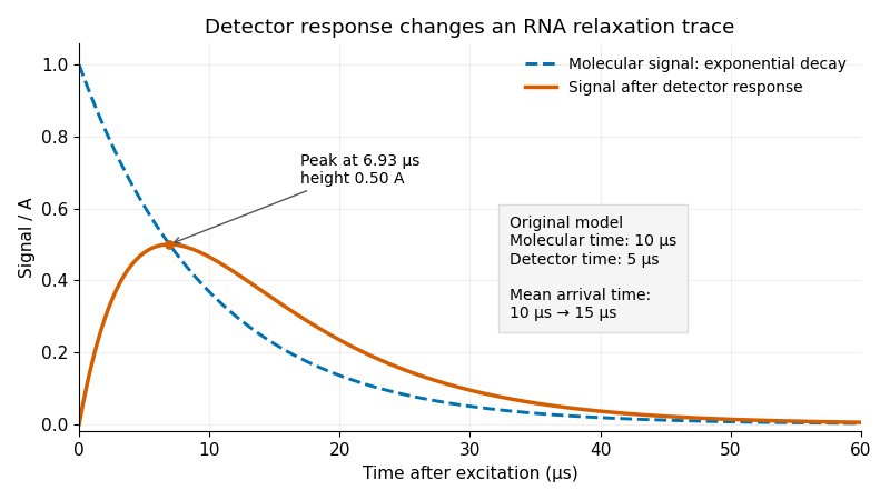
Original exponential RNA transient and its convolution with a finite instrument response function; stipulated molecular time10μs and detector time5μs
. Details. 
One useful approach predicts a molecular transient, convolves it with the characterized instrument response function, and fits that forward prediction to the data. Directly undoing a smoothing response can amplify measurement noise. Parameters that produce nearly indistinguishable recorded curves may remain difficult to determine separately.
Sample cooling is an additional physical process. A primary temperature jump study used a thin sample cell to accelerate cooling enough to observe RNA refolding, with separate infrared probe pulses following the transient.[ref]
Measuring RNA UNCG Tetraloop Refolding Dynamics Using Temperature-Jump/Drop Infrared Spectroscopy by C. P. Howe and others. Printed pp.9171–9172, thin-cell cooling and pump/probe measurement.
If temperature changes during a trace, the molecular equilibrium and rate constants may change too; detector convolution alone does not account for that changing input. The two-exponential example is a stipulated teaching model, not a fit to that paper. Articles by others on the same topic
There are currently no matching articles.