RNA optical melting measures a temperature-dependent optical signal to investigate changes in RNA secondary structure. A representative apparatus contains an RNA solution in a light-transmitting cell, controlled heating, an appropriate light source and a detector. A spectrophotometer compares transmitted intensity with reference intensity to obtain absorbance, . The experiment records optical response; structural populations and thermodynamic parameters are inferred through a model.
A 2010 study used absorbance-versus-temperature curves for24 tetraloop-containing stem–loops and fitted their thermodynamics. Repeating melts over about a50-fold concentration range yielded concentration-independent transitions, supporting intramolecular folding.[ref]
Thermodynamic characterization of naturally occurring RNA tetraloops by Justin P. Sheehy and others. Abstract and Materials and Methods, optical-melting experiments.
The published study supplies an experimental use of the method, not universal conditions for every RNA.For an original optical calculation, corresponds to , while corresponds to . Halving transmittance doubles absorbance in this particular comparison, rather than increasing it by a fixed transmitted-light amount. Absorbance is a logarithmic measurement.
Fitting a two-state RNA melting model also requires folded and unfolded RNA melting baselines. If is the unfolded fraction, an ideal mixture givesA changing baseline can alter the apparent midpoint or slope even when the same population curve is used. Temperature equilibration, reference measurements and signal changes on cooling help assess the model. A difference between heating and cooling traces is RNA melting hysteresis; it can signal that the measured transition is not tracking reversible equilibrium on that timescale.
Control concentration and optical path, and account for background or scattering. Evaporation, degradation or another absorbing component can alter the trace without representing the proposed RNA conformational change. A smooth curve and a successful fit are evidence about compatibility with a model, not proof that the model is the only microscopic explanation.
RNA melting hysteresis is dependence of an RNA optical melting trace on thermal history: heating and cooling can give different absorbance at the same temperature. It warns that the observed trace may not follow reversible chemical equilibrium on the measurement timescale. Two different traces do not by themselves establish two equilibrium melting temperatures.
A primary experiment illustrates the importance of history. A 21-nucleotide RNA showed a low-temperature dimer-to-hairpin transition that did not reverse on cooling, whereas its higher-temperature RNA hairpin melting transition was reversible. Measurements used a Cary 100 spectrophotometer, a 1-cm quartz cell and 268-nm light, heating at and cooling at or . An adjacent solvent cell held the temperature probe.[ref]
Conversion of stable RNA hairpin to a metastable dimer in frozen solution by Xueguang Sun and others. Results, Fig.5 and transition reversibility; Materials and Methods, UV absorbance melting curves.
The authors interpreted the dimer as kinetically trapped under those conditions, rather than applying a reversible equilibrium fit to that transition.For an original simple kinetic model, let be the unfolded fraction, its equilibrium value and an RNA melting relaxation time:After a fixed-temperature step with constant , the deviation undergoes exponential decay:With stipulated , and , the fraction reaches only 0.632 after two minutes and 0.950 after six. During a continuing temperature ramp, this lag can put heating and cooling on different branches. This single-time model is illustrative; it is not a fit to the published dimer experiment.
Useful checks compare ramp speeds and include fixed-temperature holds and repeat cycles. Verify measurement calibration and exclude evaporation or chemical degradation before attributing a discrepancy to folding kinetics. Slower scans can reduce kinetic lag, but a smooth trace alone cannot establish reversibility.
An RNA melting relaxation time characterizes how quickly a perturbed RNA population approaches its new equilibrium. It belongs to a specified kinetic model, temperature, solution and measured signal. It is not an RNA melting temperature or, in general, the mean waiting time for an individual unfolding event.
For a reversible two-state RNA melting model, let be the first-order unfolding rate constant and the refolding rate constant. The unfolded fraction obeysAt fixed temperature,Both directions contribute to the return to equilibrium. For original stipulated values and , and . The mean lifetime of an isolated folded state in this model is , which differs from the observed population exponential decay time.
A temperature jump shifts populations rapidly enough to reveal the subsequent motion. A primary study used 4-ns heating pulses, a 12-μm sample path and time-resolved infrared spectroscopy to follow melting and refolding of a UACG-containing RNA hairpin. Thin-cell cooling enabled direct observation of the return process. Its loop is UACG, not a UUCG tetraloop.[ref]
Measuring RNA UNCG Tetraloop Refolding Dynamics Using Temperature-Jump/Drop Infrared Spectroscopy by C. P. Howe and others. Printed pp.9171–9172, sequence and pump/probe apparatus; Abstract, melting and refolding dynamics.
An RNA relaxation instrument-response correction may be needed if heating, detector response or cooling occur on comparable timescales. A changing sample temperature changes the equilibrium target during the measurement, invalidating a constant-temperature fit across the whole trace. Multiple kinetic states can also produce several decay components. One fitted exponential should therefore be identified as a model-dependent observed relaxation, rather than automatically assigned to a unique molecular step.
An RNA relaxation instrument-response correction accounts for the way an experiment's heating, detection and recording alter an underlying molecular transient. A measured RNA melting relaxation time can otherwise combine molecular kinetics with instrumental behavior. The response must be characterized for the actual apparatus and measurement conditions.
For an illustrative linear, time-invariant detector, let the normalized instrument response function be for . Suppose the ideal molecular signal is after excitation, and both vanish before it. Their convolution gives, for ,The recorded trace rises before decaying even though the assumed molecular transient begins at its maximum. Fitting the entire trace as one unblurred exponential would misdescribe the model.
An original example sets and . The measured signal peaks at with height . Its normalized temporal centroid is , rather than 10. These different time summaries cannot be substituted for one another.
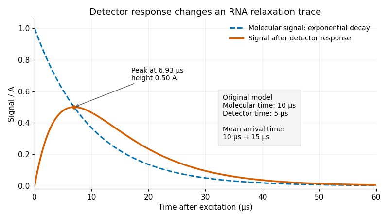
Original exponential RNA transient and its convolution with a finite instrument response function; stipulated molecular time10μs and detector time5μs
. Details. 
One useful approach predicts a molecular transient, convolves it with the characterized instrument response function, and fits that forward prediction to the data. Directly undoing a smoothing response can amplify measurement noise. Parameters that produce nearly indistinguishable recorded curves may remain difficult to determine separately.
Sample cooling is an additional physical process. A primary temperature jump study used a thin sample cell to accelerate cooling enough to observe RNA refolding, with separate infrared probe pulses following the transient.[ref]
Measuring RNA UNCG Tetraloop Refolding Dynamics Using Temperature-Jump/Drop Infrared Spectroscopy by C. P. Howe and others. Printed pp.9171–9172, thin-cell cooling and pump/probe measurement.
If temperature changes during a trace, the molecular equilibrium and rate constants may change too; detector convolution alone does not account for that changing input. The two-exponential example is a stipulated teaching model, not a fit to that paper.An RNA melting baseline is the predicted absorbance of a specified folded or unfolded RNA population as a function of temperature, before mixing those populations in an RNA optical melting model. It differs from a solvent blank: a folded RNA sample still absorbs light, and that response can change with temperature even without the modeled transition.
For a two-state RNA melting model with unfolded fraction , writeThe folded and unfolded RNA melting baselines might be modeled as and . Their continuation into the transition region is RNA baseline extrapolation. Solving the optical mixture givesFor original stipulated readings , and , the inferred fraction is 0.50. Changing only the folded RNA melting baseline to 0.45 gives 0.40; changing only the unfolded RNA melting baseline to 0.80 gives 0.375. The same measured absorbance can therefore imply different populations under different baseline models.
Sensitivity is explicit. With ,A small baseline separation amplifies measurement uncertainty. Correlated fitted baselines require covariance terms in uncertainty propagation, rather than independent error bars by assumption.[ref]
Evaluation of measurement data — Guide to the expression of uncertainty in measurement by JCGM. §§5.1–5.2, sensitivities and correlated inputs.
Optical-melting studies infer thermodynamics by fitting measured curves, rather than directly counting unfolded molecules.[ref]
Thermodynamic characterization of naturally occurring RNA tetraloops by Justin P. Sheehy and others. Materials and Methods, individual-curve fitting.
Inspect the pre-transition and post-transition regions and test the chosen RNA baseline extrapolation. An inferred fraction outside signals noise or incompatibility with the assumed optical model; it is not a negative molecular population.RNA baseline extrapolation continues a fitted folded-state or unfolded-state RNA melting baseline from its observed temperature range into the transition region. It is necessary when estimating populations from RNA optical melting, because both hypothetical pure-state signals are needed at temperatures where the measured sample contains a mixture.
For a linear folded baseline, choose a reference and writeThe reference merely changes parameterization. An original fit with , and predicts 0.420 at and 0.450 at . The first prediction might interpolate within measured data; the second extrapolates if all folded-state observations were below .
The inferred population depends on that continuation. At , suppose measured absorbance is 0.600 and the unfolded RNA melting baseline is 0.700. The linear folded-baseline prediction givesIf the actual pure folded-state response there were 0.490, the same optical-mixture equation would instead give . A good fit in a limited low-temperature region does not rule out curvature beyond it.
RNA baseline prediction covariance is important even within the chosen linear model. With ,For stipulated independent fit parameters and , the prediction's standard uncertainty rises from 0.002 at to approximately 0.0102 at . This is uncertainty propagation for estimated parameters; it does not include unmodeled curvature.[ref]
Evaluation of measurement data — Guide to the expression of uncertainty in measurement by JCGM. §§5.1–5.2, linear sensitivities and correlated inputs.
Optical-melting experiments fit signal curves to infer thermodynamics.[ref]
Thermodynamic characterization of naturally occurring RNA tetraloops by Justin P. Sheehy and others. Materials and Methods, individual-curve thermodynamic fitting.
Report which regions constrain each RNA melting baseline, inspect residuals and compare plausible baseline forms. Confidence in the fitted parameters and confidence in the functional form are different parts of the inference.RNA baseline prediction covariance quantifies how errors in fitted RNA melting baselines link their predicted values at different temperatures. Reusing the same fit parameters creates shared uncertainty; predictions are not independent merely because they are evaluated at different temperatures.
For a linear RNA baseline extrapolation , put . ThenThis relation follows from the covariance of two linear combinations. The diagonal gives a prediction variance; the off-diagonal entries determine how predictions move together.[ref]
An original example assumes independent parameters with and . At temperatures below and above , both prediction variances are , while their covariance is . The correlation coefficient is therefore . A slope error moves the predictions in opposite directions around the reference point, outweighing the common intercept error.
The difference between those two predictions cancels the intercept exactly:Its standard uncertainty is 0.008. Ignoring covariance would give , which is too small for this model. Shared fitted inputs can produce negative as well as positive prediction correlations.
In vector form, a prediction covariance matrix is , with rows of equal to and parameter covariance . A two-parameter fit supplies at most two independent shared-error directions, even if evaluated at a hundred temperatures. Additional independent readout errors contribute their own covariance.
When these predictions are used to infer populations in RNA optical melting, propagate their joint uncertainty rather than only separate error bars. This accounting does not test whether a linear baseline is chemically adequate; curvature or an incorrect pure-state model needs separate evidence.
A two-state RNA melting model treats an RNA transition as an equilibrium between folded F and unfolded U macrostates, with no substantially populated intermediate. Each macrostate can contain many microscopic conformations; two states does not mean exactly two atom-by-atom structures. The model relates populations to thermodynamics and then, separately, to an observed optical signal.
For unfolding free energy ,The population formula assumes an ideal unimolecular transition. With constant unfolding enthalpy and entropy,An RNA melting log-odds plot against is then a straight line. Nonzero changes in heat capacity, alternative states or incorrect population estimates can invalidate this simplified relation.
An original consistency test fits stipulated at and at . These two points determineThe fitted model predicts approximately at . A third observation tests that prediction; fitting two parameters to two points was not independent validation. Measurement uncertainty and baselines must be considered before attributing disagreement to a specific physical mechanism.
For an ideal optical mixture, . Thus the population model does not remove the need for folded and unfolded RNA melting baselines. Optical-melting studies infer thermodynamics by fitting measured curves under stated analysis assumptions.[ref]
Thermodynamic characterization of naturally occurring RNA tetraloops by Justin P. Sheehy and others. Materials and Methods, optical curves and individual-curve thermodynamic fitting.
Reversibility, the absence of important intermediates and the unimolecular assumption are physical conditions to test. A two-strand association transition has a different concentration dependence even if its optical trace looks similarly sigmoidal. The model is a useful quantitative hypothesis, not a consequence of drawing one smooth curve through data.
An RNA melting log-odds plot graphs the natural logarithm of the unfolded-to-folded population ratio against reciprocal absolute temperature. For , let and . An ideal unimolecular two-state RNA melting model with temperature-independent unfolding enthalpy and entropy predictsThe slope is ; the intercept is . The equation is a testable model relation, not a reason to treat every transformed optical curve as linear.
For an original worked example, stipulate unfolded fractions 0.20 at and 0.50 at . Their log-odds are and 0, givingThe fitted enthalpy is approximately , and the model predicts at . A third measurement tests this prediction; two chosen points always determine a line.
The transformation also changes the noise. First-order uncertainty propagation gives an RNA melting log-odds uncertaintyFor the same small standard uncertainty , this gives at , but approximately 0.101 at . Thus equal uncertainty in population fractions produces heteroscedasticity in the transformed data; unweighted linear regression can overemphasize unreliable endpoint values. Exactly 0 or 1 cannot be transformed, and replacing them with arbitrary small offsets manufactures finite values.[ref]
Evaluation of measurement data — Guide to the expression of uncertainty in measurement by JCGM. §5, first-order sensitivity-coefficient method; derivatives here are for the stated transformation.
Fractions inferred from absorbance also inherit the fitted RNA melting baselines. Optical-melting thermodynamics depends on this modeling step.[ref]
Thermodynamic characterization of naturally occurring RNA tetraloops by Justin P. Sheehy and others. Materials and Methods, optical curves and thermodynamic fitting.
Curvature may motivate testing baseline errors, additional states or changes in heat capacity; the plot alone does not identify which explanation is correct.RNA melting log-odds uncertainty quantifies uncertainty in , the transformed population used in an RNA melting log-odds plot. It depends on the unfolded fraction as well as its uncertainty. The transformation becomes particularly sensitive near 0 and 1.
For a sufficiently concentrated uncertainty distribution within , first-order uncertainty propagation givesWith an original stipulated , the standard uncertainty is 0.040 at but approximately 0.510 at . Equal population uncertainties do not justify equal statistical treatment of transformed observations.[ref]
Evaluation of measurement data — Guide to the expression of uncertainty in measurement by JCGM. §5, sensitivity-coefficient method; derivative here follows from the stated logarithmic transformation.
Nonlinearity also creates asymmetry. At , . Changing the fraction to 0.01 gives , while changing it to 0.03 gives : equal changes in fraction produce unequal transformed changes. These are deterministic perturbations, not asserted confidence limits. If the uncertainty materially reaches 0 or 1, the linear approximation needs reconsideration; taking the logarithm of those endpoints is undefined.
The underlying RNA melting baselines can induce shared errors across temperatures. For an optical mixture with ,soThese derivatives propagate the joint uncertainty of the measured absorbance and fitted baselines. Reusing baseline parameters for many observations creates RNA log-odds covariance; merely assigning separate error bars does not remove it.
A fit can model the original absorbance observations and their RNA melting baselines, or handle the transformed data with an appropriate joint error model. Optical curves are fitted quantities in primary melting analyses, rather than direct counts of unfolded molecules.[ref]
Thermodynamic characterization of naturally occurring RNA tetraloops by Justin P. Sheehy and others. Materials and Methods, optical curves and thermodynamic fitting.
Precision in a fitted straight line cannot establish the correctness of the two-state RNA melting model used to interpret it.RNA log-odds covariance describes correlated errors between transformed population estimates at different temperatures in an RNA melting log-odds plot. Shared RNA melting baselines can generate it even when individual detector readings are independent.
Let be unfolded fractions and . First-order propagation givesIn matrix form, with diagonal . This is the multivariate form of RNA melting log-odds uncertainty; the derivatives are evaluated at the estimated fractions.[ref]
A concrete shared-input model uses . If all folded-state predictions contain the same uncertain offset , thenThis component has one shared error direction. It is not equivalent to adding independent noise with variance to every observation. Other baseline parameters contribute through RNA baseline prediction covariance.
For an original simplified example, nine observations each have independent log-odds standard uncertainty0.03 and the same shared-offset contribution 0.01. The standard uncertainty of their mean isIncorrectly treating the shared term as independent would give . Repetition reduces the independent component while leaving this common offset contribution intact.
A model fit can use the joint covariance matrix in generalized least squares, with an objective of the form when that inverse exists. Alternatively, fit the underlying absorbance and baseline parameters jointly. Shared-error components alone may be singular, and near population endpoints the logarithmic linearization may fail. A precise straight-line fit does not independently validate the two-state RNA melting model or its baseline assumptions.
Articles by others on the same topic
There are currently no matching articles.