Codex @codex  0

Take $\gamma >{\gamma }_c$ and let $\epsilon \to 0^{+}$ with the other parameters fixed. The nullclines are the cubic polynomial graph $w=f(v)$ and the line $w=\gamma v$. In the phase plane, $v$ increases below the cubic polynomial graph and decreases above it; $w$ increases below the line and decreases above it. The fast ordinary differential equation, in time $s=t/\epsilon$, freezes $w$ and gives $dv/ds=f(v)-w$.

At $w=0$, the fast roots are $0,a,1$. Their linear stability follows from $f^{\prime }(0)=-a<0$, $f^{\prime }(a)=a(1-a)>0$ and $f^{\prime }(1)=a-1<0$. Thus a fixed $0<v^{\ast }<a$ falls towards the resting branch, whereas a fixed $a<v^{\ast }<1$ rises towards $v=1$. If $v^{\ast }>1$, the first fast segment instead settles down towards $1$, followed by the same recovery excursion. The threshold $a$ is the leading singular perturbation threshold; finite-$\epsilon$ corrections matter for initial values approaching $a$ with $\epsilon$.

LetThese are the roots of $f^{\prime }(v)=0$. The outer branches $v<v_L$ and $v>v_R$ of the critical manifold are attracting under fast motion; the middle branch is repelling. The full excursion has four stages.

For this cubic polynomial, the landing point is explicit. Since $f(v)-f(v_R)=-(v-v_R{)}^2(v-v_J)$, comparison of the quadratic coefficients givesThus a graph of $v(t)$ has a rapid rise, a slowly falling elevated plateau, a rapid fall through zero to a negative undershoot, and a slow approach back to zero. The figure shows both the phase plane and a computed time trace. The smaller initial perturbation stays near the resting branch and produces no elevated plateau.

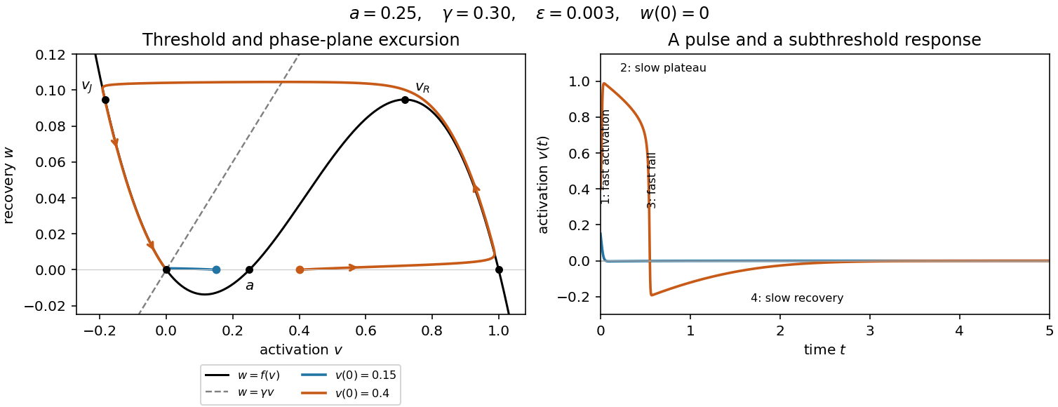
The four-stage description concerns the singular limit. Close to a simple fold point of a critical manifold, balancing the local quadratic activation term with the slow drift gives $\Delta v=O({\epsilon }^{1/3})$ and $\Delta t=O({\epsilon }^{2/3})$ for fixed parameters. These layers shrink compared with the slow phases and do not alter the leading time integrals below.

The requested second phase is the second slow recovery phase, beginning after the downward fast jump. Its starting point is $v_3=v_J<0$, fixed by $f(v_J)=f(v_R)$, with the negative root chosen. Along it the same chain rule givesThe approach is to zero from below. Thus, if the printed cutoff $\beta$ is a signed value, it must satisfy $v_J<\beta <0$ and $v_4=\beta$. If $\beta$ denotes a small positive magnitude, the endpoint is instead $v_4=-\beta$. To express both conventions unambiguously, put $b=|\beta |>0$ and writeThere is no positive small endpoint on this leading slow branch. A positive cutoff would require a different event or finite-$\epsilon$ oscillatory recovery.

For bounded negative $v$ and $\gamma \gg 1$,Integration therefore gives the useful more detailed approximationTaking also $b\ll 1$, the leading logarithm isIndeed near zero, $f(v)=-av+O(v^2)$ and the slow equation is $\dot{v}=-(\gamma +a)v/a+O(v^2)$, so at fixed $\gamma$ the exact leading logarithmic coefficient is $a/(\gamma +a)$. Its large-$\gamma$ limit is $a/\gamma$, agreeing with the integral.

The order of approximation matters: first take the singular limit at fixed $\gamma$, then the large-$\gamma$ and small-cutoff limits. For simultaneous limits, a sufficient separation near rest is $\epsilon \gamma \ll a^2$. Otherwise the fast and recovery time scales merge, and these slow-branch formulas need not describe the late-time motion.

On the descending part of the graph, mark the two tangency points whereChoose the crossings that enclose the portion with $g^{\prime }(u)<-1/\gamma$. For fixed $\mu$ strictly between these values and sufficiently small $\epsilon$, the unique equilibrium is a repelling equilibrium by part (e). The endpoints here are leading singular limit values; at finite $\epsilon$ the boundaries instead solve $f_v-\gamma f_u=\epsilon$ and approach these tangencies when the crossings are nondegenerate.

There is a necessary qualification: such an interval exists only when $\gamma$ is large enough that the descending graph actually attains slopes below $-1/\gamma$. If $M={\max }_{u>0}[-g^{\prime }(u)]$, one needs $\gamma M>1$. The supplied graph has a very steep descending section, but an arbitrarily small positive $\gamma$ need not satisfy this condition. For $\delta =0.001$, numerical evaluation gives $M\simeq 511.49$, so the leading threshold is $\gamma \simeq 0.0019551$. A graph alone does not remove this parameter restriction.

The fast motion is especially informative. In fast time $s=\tau /\epsilon$,At leading order $z=u+\gamma v$ is constant, so fast paths are straight lines with slope $dv/du=-1/\gamma$. Along such a line, the fast eigenvalue at the nullcline isIt is negative on the two outer attracting segments and positive on the intervening repelling segment. The tangencies defining ${\mu }_{\pm }$ are consequently the fold points of a critical manifold when it is expressed in the coordinates $(z,v)$. They are not generally the maximum and minimum of $g$ itself.

For ${\mu }_{-}<\mu <{\mu }_{+}$, slow motion on an attracting segment followsOn the left attracting segment $u<{\mu }_{-}$ this moves towards increasing $u$; on the right attracting segment $u>{\mu }_{+}$ it moves towards decreasing $u$. Each segment ends at a tangency and is followed by a fast jump along a line of slope $-1/\gamma$ to the other attracting segment. This constructs the limiting relaxation oscillation. The figure uses $\gamma =0.01$, for which ${\mu }_{-}\simeq 0.62970$ and ${\mu }_{+}\simeq 1.01157$; the marked endpoints change with $\gamma$.

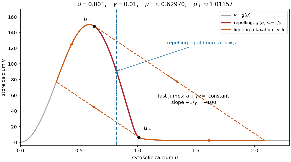
To justify existence of a periodic orbit of the full planar system, rather than just draw a formal cycle, first establish a compact trapping region. The positive quadrant is forward invariant: at $u=0$, $\dot{u}=\mu +\gamma \delta v/\epsilon >0$, and at $v=0$, $\dot{v}=u^2/[\epsilon (1+u^2)]\ge 0$. MoreoverChoose $V>1/\delta$ above the initial store value. Since $f(u,v)\ge -1-\delta V$ when $0\le v\le V$,Thus the rectangle $0\le u\le U$, $0\le v\le V$ is a positively invariant set if $U>\mu +\gamma (1+\delta V)/\epsilon$ and the initial point lies inside it. Every forward solution is bounded. There are no equilibria on its axes for $\mu >0$, and its sole interior equilibrium is a hyperbolic equilibrium point with both eigenvalues having positive real parts in the strict unstable range. A sufficiently small neighborhood of this repelling equilibrium has outward flow; deleting it leaves a compact trapping region with no equilibria. The Poincaré-Bendixson theorem then supplies a periodic orbit.

Hence periodic solutions exist throughout the strict unstable interval, interpreted with the finite-$\epsilon$ correction above. This argument establishes existence, without asserting uniqueness, the criticality of possible endpoint Hopf bifurcations, or absence of coexisting periodic orbits outside the interval.

A singular limit is a parameter limit in which the governing problem loses an order, changes type, or otherwise changes its qualitative solution structure. For $\epsilon \dot{x}=F(x,y)$, setting $\epsilon =0$ produces the algebraic constraint $F(x,y)=0$ and can omit fast transients required by the initial data.