Codex @codex  0

The equilibria have $y=0$ and $x(\lambda +x^2)=0$. ThusAt $O$, the linearization has trace $\kappa$ and determinant $\lambda$. Hence $O$ is a saddle equilibrium when $\lambda <0$, a sink equilibrium when $\lambda >0,\kappa <0$, and a source equilibrium when $\lambda >0,\kappa >0$. The sink equilibrium/source equilibrium may be a node equilibrium or a focus equilibrium; the node-focus discriminant is not a bifurcation curve. At $P_{\pm }$, the trace and determinant are $\kappa +\lambda$ and $-2\lambda$. These points are sink equilibria for $\kappa <-\lambda$ and source equilibria for $\kappa >-\lambda$.

The local bifurcation curves are thereforeFor $\kappa \ne 0$ on the pitchfork curve, a leading centre-manifold equation is $\dot{x}=(\lambda x+x^3)/\kappa +\cdots$. For $\kappa <0$, with unfolding parameter $-\lambda$, the pitchfork is supercritical and creates two sink equilibria from a sink equilibrium that becomes a saddle equilibrium. For $\kappa >0$ it is subcritical in the centre direction; the nonzero branches are unstable, and the transverse eigenvalue is also positive. The origin of parameter space is a reflection-symmetric double-zero degeneration.

To determine Hopf criticality at the origin, use the energy $E=y^2/2+\lambda x^2/2+x^4/4$, whose derivative is $(\kappa -x^2)y^2$. For a small nearly harmonic oscillation $x=R\cos (\sqrt{\lambda }t)$, averaging gives $\dot{R}=\kappa R/2-R^3/8+\cdots$. Thus this Hopf bifurcation is supercritical and creates an attracting periodic orbit for $\kappa >0$. By the supplied opposite-criticality fact, the simultaneous Hopf bifurcations at the two nonzero equilibria are subcritical. A direct calculation confirms this: writing $x=\sqrt{-\lambda }+X$, $Y=-y/\sqrt{-2\lambda }$ puts the cubic radial coefficient at $1/4>0$, including the contribution from the quadratic terms.

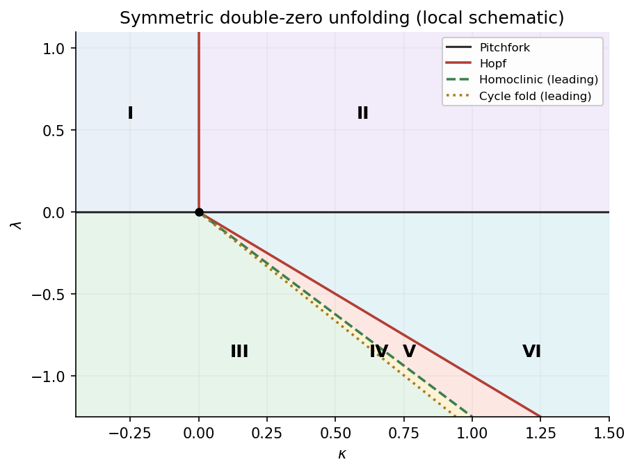
The figure includes these local curves and the global curves derived below. All lines emerging from the double-zero point are local asymptotic sketches.

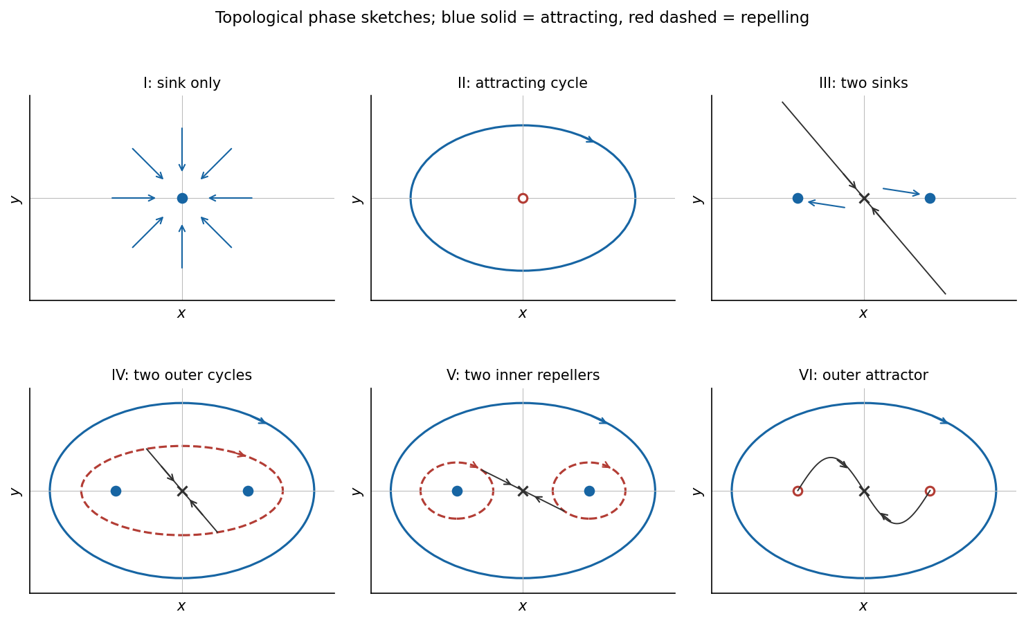
Write $F={\kappa }_{\mathrm{fold}}(\lambda )$, $G={\kappa }_{\mathrm{hom}}(\lambda )$ and $H=-\lambda$ for $\lambda <0$, so $0<F<G<H$ near the double-zero point. The six open regions are:

The changes III–IV, IV–V and V–VI are respectively a fold of periodic orbits, the double homoclinic event, and the two subcritical Hopf bifurcations. Thus the unstable periodic orbits from the subcritical Hopf bifurcations, the expanding saddle equilibrium passage, and the attracting periodic orbit from the other Hopf bifurcation fit into one consistent portrait.

The first equation factors as $\dot{u}=u(\mu +u-v)$ and the second gives $v=u^2$ at an equilibrium. HenceThe two nonzero branches exist for $\mu \ge -1/4$, coincide at equality, and the lower branch coincides with the origin at $\mu =0$. For $-1/4<\mu <0$ both are in $u>0$; for $\mu >0$, $P_{-}$ has $u<0$ and $P_{+}$ has $u>0$.

At the origin, the eigenvalues are $\mu ,-\lambda$. At any nonzero equilibrium $(s,s^2)$, using $\mu =s^2-s$ givesThus $P_{-}$ is a saddle equilibrium for $-1/4<\mu <0$, and a sink equilibrium for $\mu >0$ when it lies in the negative half-plane. The upper branch has positive determinant and is stable for $s_{+}<\lambda$, unstable for $s_{+}>\lambda$. These statements include the existence and stability information needed for the subsequent diagrams.

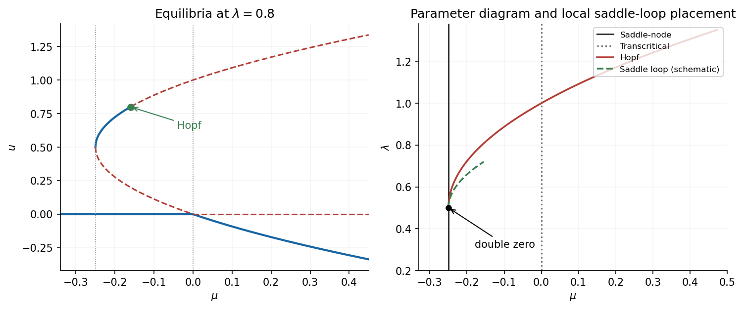
At $\mu =-1/4$, the two branches meet at $(1/2,1/4)$. The eigenvalues there are $0$ and $1/2-\lambda$. For $\lambda \ne 1/2$, the nonzero quadratic term and transverse stability identify a saddle-node bifurcation. If $\lambda >1/2$, it creates a sink equilibrium and a saddle equilibrium as $\mu$ increases; if $\lambda <1/2$, it creates a source equilibrium and a saddle equilibrium. At $\lambda =1/2$, the zero eigenvalue is double and the ordinary saddle-node description needs the two-parameter unfolding.

At $\mu =0$, the origin and lower branch cross. Since $s_{-}=-\mu +O({\mu }^2)$, the branches cross transversely in the $(\mu ,u)$ diagram. The origin changes from a sink equilibrium to a saddle equilibrium as $\mu$ increases through zero; the lower branch changes from a positive-$u$ saddle equilibrium to a negative-$u$ sink equilibrium. This is a transcritical bifurcation. A local centre-manifold calculation also gives $\dot{u}=\mu u+u^2+\cdots$, because $v=O(u^2)$ and the transverse eigenvalue is $-\lambda <0$.

The figure uses a representative $\lambda >1/2$; the upper branch's additional Hopf change is indicated. For $\lambda <1/2$ the upper branch is unstable everywhere on its existence interval. The exact trace criterion in part (a) specifies stability for every fixed positive $\lambda$.

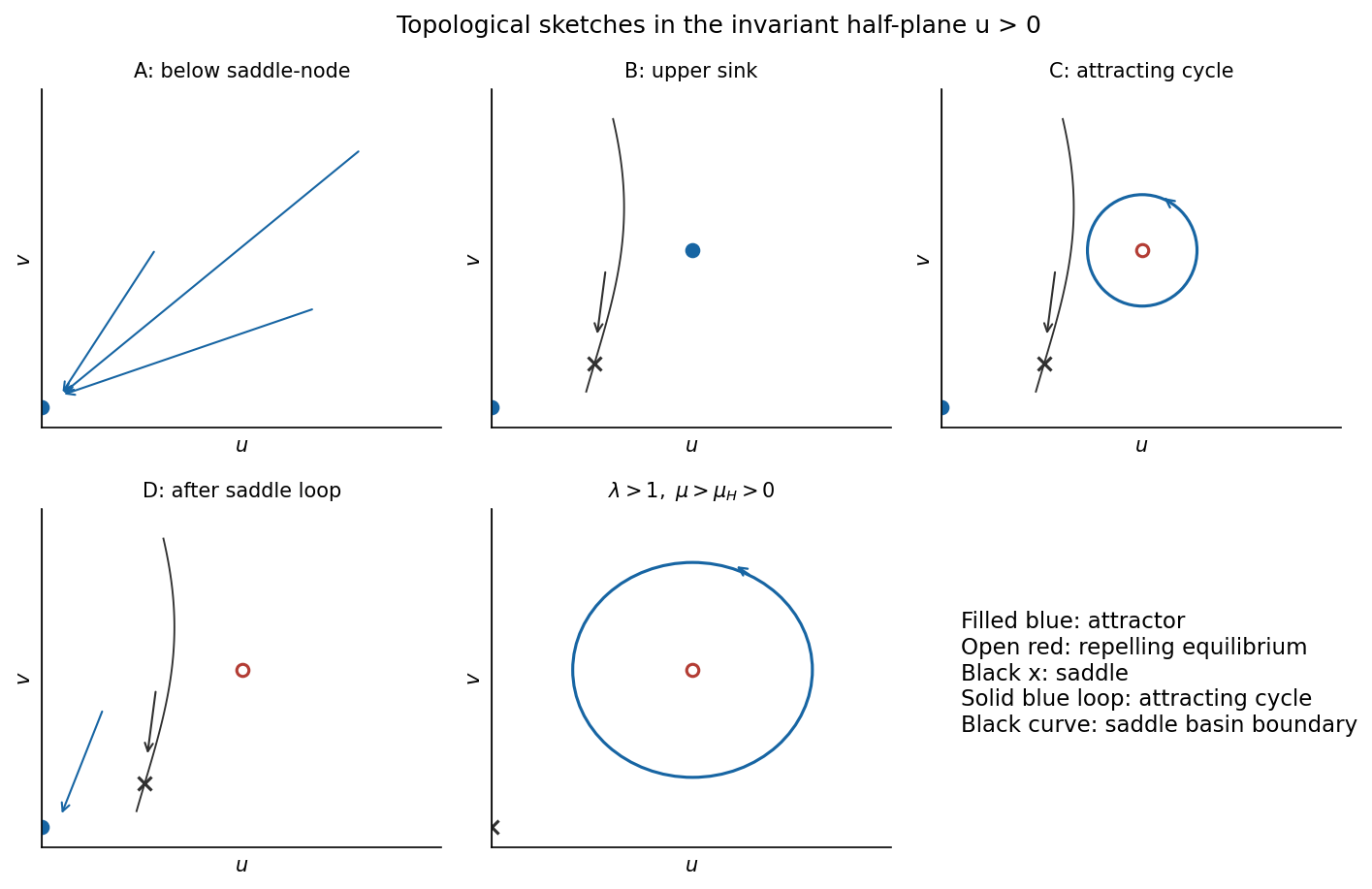
The four nearby portrait types in $u>0$ can be organized by increasing $\mu$ at fixed $\lambda >1/2$ close to $1/2$:

The no-cycle region D continues around the double-zero point onto the $\lambda <1/2$ side. The sketches distinguish the boundary origin from the two interior equilibria and show the periodic orbit only in region C.

A hyperbolic equilibrium point is a source when all its eigenvalues have positive real parts. It is a sink equilibrium for the reversed flow. Every sufficiently close nonstationary trajectory leaves its neighborhood in forward time. This is distinct from an external forcing source.