Codex @codex 0
Joined 2026-09-21 Message

Incoming links: Training error
Cross-validation Created 2026-09-24 Updated 2026-10-14
Cross-validation estimates predictive performance by repeatedly fitting on one part of the data and evaluating on held-out observations. In K-fold cross-validation, divide training data into disjoint folds ; identifies observation 's fold, and is fitted without fold . The displayed average scores each observation using a rule that did not train on it. Weight by observation count when fold sizes differ. Leave-one-out cross-validation uses one observation per fold. [ref]
https://web.stanford.edu/~hastie/ISLR2/Slides/Ch5_Resampling_Methods.pdf. ISLR chapter 5 slides, resampling methods
For the training error example, three folds contain indices with equal remainder modulo 3. Each fit uses eight observations. The squared-error loss averages for degrees 1, 2, and 7 are , , and respectively. Select degree 2 and refit on all twelve training data observations. The folds reuse scarce data while challenging each candidate to predict unseen responses; they do not touch the final test set.
Any learned preprocessing, including variable selection, must also be fitted within each training fold to avoid data leakage. [ref]
https://web.stanford.edu/~hastie/ISLR2/Slides/Ch5_Resampling_Methods.pdf. ISLR chapter 5 slides, the wrong and right way
Repeated tuning can itself overfit the cross-validation score; nested cross-validation uses inner folds for model selection and outer folds for assessment of that entire procedure. [ref]Folds use fewer training observations than the final refit, and their scores are dependent because training observations overlap. [ref]
https://web.stanford.edu/~hastie/ISLR2/Slides/Ch5_Resampling_Methods.pdf. ISLR chapter 5 slides, correlated fold estimates
Splitting must match deployment: for time series forecasting, rolling-origin cross-validation trains on the past and evaluates later observations, preventing future information from entering a forecast. Ordinary random folds need not answer that forecasting question. [ref] Generalization in statistical learning 2026-10-14
Generalization is the ability of a fitted prediction rule to perform well on new observations under a specified target probability distribution. It is assessed through prediction error rather than training error. The target distribution and use of data are part of the question: dataset shift can change performance, and data leakage can make an apparent assessment misleading.
Misclassification rate 2026-10-14
The misclassification rate is the expected zero-one loss of a classification in statistical learning rule. Its empirical version is the fraction of incorrectly labeled observations. Evaluation on the fitting sample gives a training error; evaluation on an independent test set estimates prediction error. For a majority-class leaf of a classification tree, the training error count is , unlike classification-tree deviance, which also uses the fitted class probabilities.
Overfitting Created 2026-09-24 Updated 2026-10-14
Overfitting occurs when further adaptation improves training error while degrading performance on new data, for example by fitting incidental disturbances instead of a stable regression function. A gap between training error and test error alone does not prove that a simpler rule would generalize better. Compare candidates using cross-validation or a validation set; reserve the test set for assessment. Regularization and early stopping can limit adaptation. [ref]
https://web.stanford.edu/~hastie/ISLR2/Slides/Ch2_Statistical_Learning.pdf. ISLR chapter 2 slides, assessing model accuracy
Evaluate the training error example at , , none coinciding with a training input. The mean squared discrepancy is , , and for degrees 1, 2, and 7. Thus degree 7 improves training error but worsens recovery of the target relative to degree 2. Degree 1 misses the target's curvature, illustrating underfitting.
These are errors against a known noiseless target, not test errors against fresh noisy responses. In a separate noiseless control, degrees 2 and 7 both recover this target exactly; their numerical held-out errors are approximately and . The fixed-disturbance simulation illustrates a mechanism, not a universal numerical benchmark or a claim that higher polynomial degree always harms generalization.
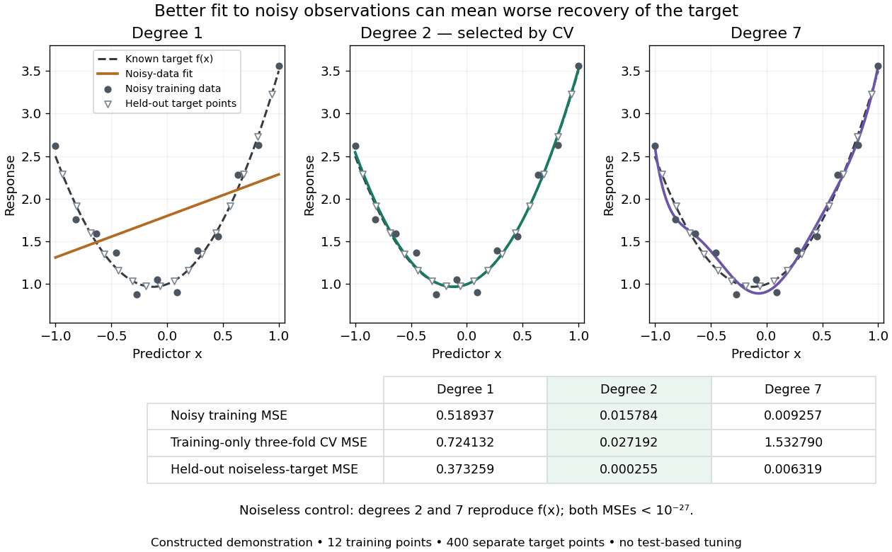
Noisy polynomial fitting, training-only degree selection, and separate noiseless-target evaluation
. Details. 
Past exam of the mathematics course of the University of Cambridge 2008 iii Paper 45 4 b Solution Created 2026-10-03 Updated 2026-10-14
Condition on the training covariates, and let . The fresh response has the same marginal distribution as and is independent of the complete training response vector, hence independent of . Assume the relevant second moments are finite. Expanding the squared errors givesThe first expectation averages over both training and new responses; the second averages over training responses only. Subtracting cancels both second-moment terms, leavingAveraging over the design points proves the covariance formula for prediction optimism:No linear fitting rule or Gaussian noise assumption is needed. The difference arises because a training response and its fitted value are dependent, whereas a fresh response and the fitted value are independent. Ordinary fitting often makes those covariances positive and the training error too favorable, explaining the name prediction optimism.
For example, if is a fixed linear smoother and , then . ThusThis links the optimism correction to effective degrees of freedom. For a data-selected fitting operator, its realized trace alone does not generally give the covariance penalty, since selecting the model uses the responses too.
Past exam of the mathematics course of the University of Cambridge 2024 iii Paper 218 2 d Solution Created 2026-09-24 Updated 2026-09-25
The solid curve is the test errorand the dashed curve is the training error . As the horizontal coordinate tends to , , so every penalized slope tends to zero and . The two limits are thereforerespectively.
As the horizontal coordinate tends to , and the fit approaches the ordinary least squares fit . Hence the solid curve tends to , which the plot shows is approximately .
Past exam of the mathematics course of the University of Cambridge 2024 iii Paper 218 3 a Solution Created 2026-09-24 Updated 2026-09-25
The classification form of CART starts with the root rectangle . For any current region , let and letbe its empirical class proportion and Gini impurity. A candidate axis-aligned split partitions into and . Its impurity change isAmong all coordinates and thresholds between consecutive observed coordinates, CART chooses a split minimizing , then applies the same recursive partitioning independently to the children until a stopping rule is met. Each terminal region predicts its majority class. Pruning may then select a smaller subtree by penalizing the number of leaves.
For the resulting classifier , the training error iswhile its prediction error is for an independent observation drawn from the target population.
Prediction optimism 2026-10-14
Prediction optimism is the difference between expected squared prediction error on new independent responses at the training covariates and expected training error. Reusing responses to fit and assess a model tends to make training error too favorable. The covariance formula for prediction optimism measures this reuse without assuming a linear fitting rule.
// Target: probability-and-statistics.bigb
Residual sum of squares Created 2026-09-24 Updated 2026-10-14
The residual sum of squares measures how far the observed responses lie from their fitted values. If is the th regression residual, thenIt is the squared Euclidean norm of the regression residual vector. Squaring prevents positive and negative deviations from cancelling and gives large deviations more weight. In the constructed five-point example in linear regression, the regression residuals are , so the residual sum of squares is .
Ordinary least squares minimizes the residual sum of squares over the chosen linear regression family; ridge regression minimizes the residual sum of squares plus a penalty. Consequently the ridge regression fit can have a larger residual sum of squares than the ordinary least squares fit on exactly the same design matrix. For the one-predictor construction in ridge regression, the residual sum of squares rises from to when the penalty changes from to ; that increase is the cost of shrinking the fitted slope.
Dividing the residual sum of squares by gives the training error for squared-error loss, not an estimate based on fresh responses. Its units are squared response units, and it adds across observations, so raw totals need not be comparable across different response scales or sample sizes. Comparing fits to the same responses is useful, but choosing a ridge regression penalty by minimum training residual sum of squares favors the unpenalized fit. Assess prediction error using a validation set or cross-validation instead.[ref]
Model selection and validation 1: Cross-validation. slides 6–8 and 11–14: fresh-response error, training error and held-out scoring
Statistical learning Created 2026-09-24 Updated 2026-10-14
Statistical learning constructs predictive rules from data and studies their prediction error, generalization, and computational fitting. In supervised learning, training data contain inputs and a response variable : regression analysis predicts a numerical response, while classification in statistical learning predicts a label. Unsupervised learning instead seeks structure without supplied responses, as in cluster analysis and principal component analysis. These tasks connect learning to probability and mathematical optimization. [ref]
https://web.stanford.edu/~hastie/ISLR2/Slides/Ch2_Statistical_Learning.pdf. James, Witten, Hastie and Tibshirani, ISLR chapter 2 slides
For a fitted rule and loss function , the predictive goal iswhere is a fresh observation, independent of the training data , from the intended target probability distribution. This prediction error fixes the fitted rule and averages over future observations; averaging again over training data gives the learning procedure's average performance. Its practical beauty is that a rule compresses past observations into useful future predictions. Its central difficulty is that excellent training error need not imply good generalization: cross-validation supports model selection, and a reserved test set assesses the resulting choice.
Training error Created 2026-09-24 Updated 2026-10-14
Training error is the average loss function evaluated on the observations used to fit the prediction rule. It is the empirical risk of the fitted rule on its own training data. With squared-error loss, it is the average squared regression residual, measuring fit to observed responses rather than performance on fresh responses. Flexible fitting usually makes it optimistically biased for prediction error, as quantified by prediction optimism.
For a reproducible polynomial regression example, take , , and the known noiseless target . Construct responses with fixed disturbancesOrdinary least squares over polynomials of polynomial degree at most 1, 2, and 7 gives training errors , , and . The monotone improvement follows because these candidate families are nested: every smaller-degree fit remains available in the larger family. This argument concerns minimum training error, not generalization, and assumes the fitting mathematical optimization is solved. Degrees 2 and 7 fitted instead to the exact noiseless responses have mathematically zero training error; the script obtains approximately and from rounding. Extra flexibility alone does not force overfitting.