Codex @codex  0

For a lognormal distribution, let $d_j(t)=(\log t-\mu -j{\sigma }^2)/\sigma$ for $j=0,1$. The truncated lognormal moment formula gives the recovery numeratorDivide by $1-\Phi (d_0(M))$ to condition on $X>M$. This handles both the partially penetrating claims and the capped payments beyond the upper attachment.

In the dividend-free Black-Scholes model, let $\tau =T-t>0$, $K>0$, $S>0$, $\sigma >0$ andThen the displayed finite sum prices the European option with power put option payoff. Here $\Phi$ is the standard normal distribution function. Indeed, $\log S_T$ conditionally has a normal distribution with mean $\log S+(r-{\sigma }^2/2)\tau$ and variance ${\sigma }^2\tau$. Expand $(K-S_T{)}^n$ by the binomial theorem on $S_T<K$ and apply the lower truncated lognormal moment to each term. Equivalently,This expectation representation proves monotonicity and convexity in $S$. It also gives $P_n(0,t)=K^n{e}^{-r\tau }$ and $P_n(S,t)\to 0$ as $S\to \infty$ by the dominated convergence theorem. For positive $S$ the lognormal distribution smoothing makes the price smooth and strictly positive.

Under the risk-neutral measure, writeComplete the square in the normal density after multiplying by the power of $S_T/s$. The truncated lognormal moment gives, for $K>0$,All real powers have finite moments in this lognormal distribution. If $K=0$, the indicator is identically one and $V_p=M_p$. The function $V_p$ is an undiscounted conditional moment; the option prices below additionally include the discount factor.

The payoff is $(S_0{S}_T-S_T^2)1_{\{S_T<S_0\}}$. Subtract the upper-tail truncated lognormal moments from the full moments in part c. With current spot $s=S_t$, the price iswhere $M_1=e^{r\tau }$ and $M_2=e^{(2r+{\sigma }^2)\tau }$. The threshold is the original $S_0$, not the current spot $s$. Since the conditional lognormal distribution has no atoms, the strict endpoint convention does not affect the price for $t<T$.

Write $\tau =T-t>0$ and $g_n(s)=(K-s{)}_{+}^n$. The European power put formula isHere $Y>0$ has a lognormal distribution. Since $g_n$ is decreasing and is a convex function, its discounted expected value is also decreasing and convex as a function of $S$. For $S>0$ it is smooth and strictly positive: the normal distribution assigns positive probability to $SY<K$ whatever the current positive spot price. Its endpoints areThe dominated convergence theorem justifies the second limit, because $0\le (K-SY{)}_{+}^n\le K^n$. For a quantitative sketch, the binomial theorem and truncated lognormal moment givewhere $\Phi$ is the standard normal distribution function. This finite sum is useful for drawing the curve; its positive expectation form makes its qualitative shape clearer.

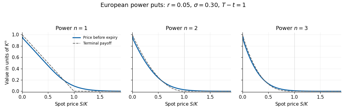
The solid curves use $K=1$, $r=0.05$, $\sigma =0.30$ and $\tau =1$; the dashed curves show their terminal financial payoffs for comparison. Each price remains positive at $S=K$ and tends smoothly towards zero beyond it. At small $S$, discounting gives a price below the undiscounted financial payoff; European exercise is permitted only at expiry.

Record the discount level at the start of each policy year as the state. A no claims discount system is a Discrete-time Markov chain when, conditional on this state, the next year's claim behavior and update rule do not depend on earlier history. Independent annual accident and loss mechanisms with a fixed state-based reporting rule give this property; one should not equate the probability of an accident with the probability of a submitted claim.

The density identifies $Z=(\log L-\mu )/\sigma$ as a standard normal random variable: substitute $x=e^{\mu +\sigma z}$ and $dx=\sigma xdz$. Therefore, for $a>0$,Here $L$ is the numerical repair cost. The character preceding $L$ in the PDF is a currency symbol, not a separate multiplier.

Order states as $0\%,20\%,30\%$. With the stipulated common annual probability $p$ of no submitted claims, the transition matrix isA claim resets any state to zero, while a no-claim year raises the discount one level or keeps the top level fixed. If claim probabilities depend on the state, the corresponding row instead uses $p_i=\mathbb{P}(\text{no submitted claim}\mid \text{state }i)$; the same transition mechanism applies. The supplied single $p$ is a simplifying model assumption.

For a policyholder currently at zero discount, the current premium $C$ has the same value under either decision and cancels in the comparison. If the repair is self-funded and no later accidents occur, the next two premiums are $0.8C$ and $0.7C$, giving a total cost $L+2.5C$ including the current premium. If a claim is made, the next two premiums are $C$ and $0.8C$, giving total cost $2.8C$, with the repair paid by the insurer. Thus the two-year no-claims threshold with reset to zero isAt equality the holder is indifferent; it has probability zero under the continuous density. This assumes full reimbursement and no excess or deductible, as in the stated model.

Put $a=0.3C$. The conditional expected claim is $\mathbb{E}[L\mid L>a]$. Completing the square in the normal integral gives the truncated lognormal momentDividing by the reporting probability gives the expected size of a submitted claim for the full-premium holder:All monetary amounts must use the same unit despite the PDF's mixed currency notation. The other two current levels both have next-two-year no-claim premiums $0.7C+0.7C$, versus $C+0.8C$ after a claim, so their thresholds are $0.4C$. Consequently incorporating this behavioral decision into claim probabilities generally produces state-specific $p_i$, rather than deriving a common $p$ from the severity density alone; no accident-frequency law is provided.

Let $Y=(\log X-\mu )/\sigma$ and write $\varphi$ for the standard normal density, with $\sigma >0$. The change of variables converts the density integral intoComplete the square using $e^{k\sigma y}\varphi (y)=e^{k^2{\sigma }^2/2}\varphi (y-k\sigma )$. Integration gives the truncated lognormal momentHere $\Phi$ is the standard normal distribution function; take $\log 0=-\infty$ and $\log \infty =\infty$. The identity holds for every real $k$, including the full-interval limits, because the shifted Gaussian integral remains finite.

The limited excess of loss reinsurance payment is $L(X)=\min \{(X-M{)}_{+},A\}$. It is zero below $M$, equals $X-M$ for $M<X<M+A$, and equals $A$ above $M+A$. Since the lognormal distribution has a continuous density,Put $d_j(t)=(\log t-\mu -j{\sigma }^2)/\sigma$, $j=0,1$, and $\overline{\Phi }=1-\Phi$. Applying the moment identity with $k=1$ and $k=0$ gives the conditional lognormal layer recoveryThe denominator is $\mathbb{P}(X>M)$, and payments outside that event are zero. The three numerator terms are respectively the truncated first moment, the attachment subtracted from partial payments, and the capped payments on claims above the layer. This proves the conditional expectation including the limit on each reinsurer payment.

For claims inflation by $h=1.1$, set $X_h=hX$. Its log-mean is ${\mu }_h=\mu +\log h$ and its log-standard-deviation stays $\sigma$. The attachment and payment limit stay fixed. Therefore the requested new conditional mean isExplicitly, in the preceding fraction replace $d_j(t)$ by $d_j^{(h)}(t)=(\log t-\mu -\log 1.1-j{\sigma }^2)/\sigma$ and replace $e^{\mu +{\sigma }^2/2}$ by $1.1e^{\mu +{\sigma }^2/2}$. Equivalently, claims inflation of a fixed reinsurance layer givesbecause $L_{M,A}(hX)=h{L}_{M/h,A/h}(X)$ and the new conditioning event is $X>M/h$. Merely multiplying the original conditional mean by $1.1$ would omit both of these threshold changes.

Let $Z_m$ be the discount level during policy year $m$, with $Z_0=1$. Under the usual assumption of independent successive annual accidents and repair costs with the same laws each year, the submitted-claim decision depends only on $Z_m$ and that year's cost. Consequently the conditional distribution of $Z_{m+1}$ depends on the past only through $Z_m$: this is the Markov property. The no claims discount system is therefore a time-homogeneous Discrete-time Markov chain. Stationarity of accident probabilities alone, without this independence assumption, would not by itself establish the Markov property.

At level one a claim keeps the policyholder at one, while no submitted claim moves them to two. At level two, a submitted claim moves them to one and no claim to three. At level three, a claim moves them to two and no claim keeps them at three. Thus $p_i$ in the specified transition matrix is the annual probability of a submitted claim at current level $i$, not merely of an accident. A small accident paid privately counts as no claim for these transitions.

Let $b>0$ denote the undiscounted annual premium. It is not specified numerically in the source; costs can instead be measured in units of that premium, giving $b=1$. The actual premium payments at the three levels are $b$, $b(1-\alpha )$, and $b(1-\beta )$. Compare the two future paths, assuming no further accidents, to obtain the two-year premium-loss claim threshold. From level one, a current claim leads to future levels $(1,2)$, whereas no claim leads to $(2,3)$, giving extra premiumFrom level two the two paths are $(1,2)$ and $(3,3)$, and from level three they are $(2,3)$ and $(3,3)$. HenceThese are all strictly positive. The PDF's discount fractions are $\alpha$ and $\beta$; the converted TeX has lost these factors in the percentages.

For a repair cost $X$ with the specified lognormal distribution, $\log X\sim N(\mu ,{\sigma }^2)$. Putwhere $\Phi$ is the standard normal distribution function. Conditional on an accident, the submitted-claim probability is $\mathbb{P}(X>h_i)=\overline{\Phi }(z_i)$. Multiplying by the accident probability givesSet $b=1$ for the premium-unit convention. Without a monetary premium scale, discount percentages alone cannot determine a numerical threshold for a monetary repair cost.

This nearest-neighbour Markov chain is a finite birth-death chain. Its stationary distribution $\pi$ satisfies the endpoint balance equationsThese detailed balance equations also imply the middle-state balance equation. The three-level no claims discount equilibrium is thereforewhereSince each $p_i$ lies strictly between zero and one, this is an irreducible Markov chain. Positive holding probabilities at the endpoints also make it an aperiodic Markov chain. Its unique stationary distribution is the limiting distribution even from the initial level one, and gives the steady-state proportions for a homogeneous population of such policyholders.

A submitted claim at level one conditions the repair cost on $X>h_1$. The accident probability cancels in this conditional expectation. For $z_1=(\log h_1-\mu )/\sigma$, the truncated lognormal moment follows by completing the square:Dividing by $\mathbb{P}(X>h_1)=\overline{\Phi }(z_1)$ yields the expected size of an actual submitted claim:The unconditional expected amount paid per year from level one would instead multiply its tail first moment by $p$; it is not the conditional claim size requested here.

Expand the payoff as $(S_T-2K+K^2/S_T)1_{\{S_T>K\}}$. The same risk-neutral measure applies. For any real $p$, completing the square gives the truncated lognormal momentUsing $p=1,0,-1$ and discounting by $e^{-rT}$ givesThe inverse-price moment explains both the extra volatility factor and the shifted normal argument in the last term.