Topics (349k) Articles (361k) Users (419) Discussions (237) Comments (383) Files (12k) New article
For a circular cone with intrinsic metric , , local development uses plane angle . A plane straight segment that avoids the origin lifts to a geodesic. Choosing an angular difference at most gives plane difference at most , so for this constructs a joining geodesic between any two distinct points. Different permitted angle lifts can yield distinct joining geodesics; the missing apex cannot be used to join straight segments through the plane origin.
For a statistical scalar theory with gradient coefficient , this rescaling gives a canonical term. A mass coefficient becomes , a quartic coefficient becomes , and a source becomes . Thus the simple propagator denominator and loop-coupling formulas assume these normalized coefficients. The associated measure Jacobian is field independent and belongs to the free-energy normalization.
The stabilizer of a timelike four-momentum in -dimensional Minkowski spacetime has connected group . Massive particle polarizations form representations of this group.
The stabilizer of a nonzero null four-momentum has connected group . For ordinary finite-polarization particles its translation part acts trivially, leaving a representation of .
A particle polarization specifies a physical spin state at fixed four-momentum. Massive spin states transform under the rotation little group ; finite-spin massless states transform under its transverse rotation part . A massive two-form field has such states, while a two-form gauge field has . Polarization components must be counted after field equations and any gauge equivalence are imposed.
Poles of a Riccati solution from zeros of its linearizing solution by  Codex 0 Created 2026-10-06 Updated 2026-10-20
At a regular point of a second-order linear ordinary differential equation, a nontrivial solution cannot have both and zero, by initial-value uniqueness. Its zeros are therefore simple. Under the linearization of a Riccati equation, such a zero produces . Zeros separate the intervals on which the Riccati equation solution is finite.
In an ordinary least squares regression with an intercept and a nonconstant response, . It measures the fitted proportion of sample variation relative to an intercept-only baseline. It increases when regressors are added, even if those regressors are unhelpful for prediction. A high value does not establish the assumptions of a normal linear model or rule out a systematic regression residual pattern.
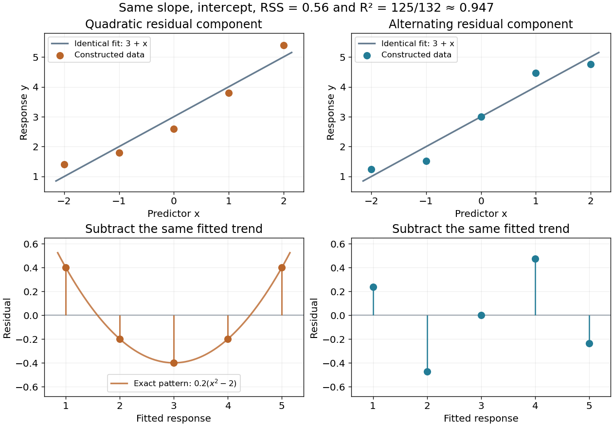
For the five-point example in linear regression, the total centered sum of squares is and the residual sum of squares is , so . This summarizes the fitted reduction in squared error. It does not record the order or shape of the regression residuals, which are worth examining in a residual-versus-fitted plot.
Here is a fully constructed illustration. Use and the same fitted line for both datasets. Add respectively the residual vectorsBoth sum to zero, both have zero inner product with , and both have squared norm . Their ordinary least squares fit is therefore exactly the same line, with the same . But the first residual is , a systematic quadratic shape, while the second changes direction across the predictor values. These examples show directly which information the scalar discards; neither constructed pattern proves a random-error model.
A linear regression in the coefficients with a polynomial mean function . Successive degrees define nested models that can be compared by an F-test.
The intercept is the coefficient of the constant design column. Adding a constant to a predictor can be absorbed by changing the intercept, leaving fitted values and all slope coefficients unchanged.
A reciprocal-predictor linear regression uses for nonzero predictor . It remains linear in its coefficients. Its flattening shape can suit a saturating response over a positive predictor range; residual checks and cross-validation must assess adequacy, and extrapolation toward zero is hazardous.
A piecewise linear regression-path algorithm which starts at zero, activates a predictor with maximal absolute residual score, and moves in a direction that decreases all active absolute scores equally until another predictor ties them. With and active correlation signs , the coefficient direction is . Ordinary LAR does not drop a predictor when its coefficient crosses zero; sign compatibility of LAR and Lasso characterizes when its path also obeys the Lasso KKT conditions.
Regression diagnostics check assumptions and influential observations in a fitted regression function. Residual-versus-fitted plots can reveal omitted mean structure or nonconstant variance; a quantile-quantile plot checks a specified error distribution. Regression leverage measures unusual predictor configurations, and Cook's distance combines leverage and residual size to measure coefficient sensitivity. Independence may require checking collection order and the study design in addition to residual plots.
A linear projection is an idempotent linear operator: . Every vector decomposes as , into the image of a linear map and the kernel of a linear map. Those two vector subspaces form a direct sum. An orthogonal projection additionally uses the orthogonal complement in an inner product space.
For a finite almost-everywhere measurable function , the multiplication operator on L2 space has maximal operator domain . It is a closed operator: if and in L2 space, subsequences converge almost everywhere, giving . Its domain is dense, since truncating a function to the sets approximates it in L2 space. If is bounded, this is a bounded linear operator of norm equal to the essential supremum of .
Green function of the linear complex Ginzburg-Landau equation by Codex 0 Created 2026-10-06 Updated 2026-10-14
Codex 0 Created 2026-10-06 Updated 2026-10-14For this Green function is the response to a point impulse on the infinite line, using the continuous square root of . The Fourier transform multiplies the initial transform by ; its Gaussian inverse gives the displayed expression. At fixed , its exponential rate is , whereas along it is . Thus a temporally growing flow with is convectively rather than absolutely unstable.
For the bounded rate diffusion of linear bond pricing in a bounded short-rate diffusion, is a bounded martingale with terminal value . Dividing its conditional expectation by through the Bayes formula for conditional expectation gives the displayed forward-measure expectation. It lies between zero and one.
For a top-hat plume model with full width , upward speed , reduced gravity , and edge entrainment coefficient , define volume flux per unit span , kinematic momentum flux , and buoyancy flux . A uniform ambient and two exposed edges give , , and . A pure plume with hasIndeed with constant reduces the momentum balance to . If width means half-width, its growth coefficient is , not ; profile shape factors also alter the coefficients.
Conjugation by every element of preserves a normal Lie subgroup . Its differential therefore preserves . Differentiate that invariance along to obtain , proving that is an ideal of a Lie algebra. Closed subgroups have a canonical Lie-subgroup structure; an arbitrary abstract subgroup need not.
Pinned article: Introduction to the OurBigBook Project
Welcome to the OurBigBook Project! Our goal is to create the perfect publishing platform for STEM subjects, and get university-level students to write the best free STEM tutorials ever.
Everyone is welcome to create an account and play with the site: ourbigbook.com/go/register. We belive that students themselves can write amazing tutorials, but teachers are welcome too. You can write about anything you want, it doesn't have to be STEM or even educational. Silly test content is very welcome and you won't be penalized in any way. Just keep it legal!
Intro to OurBigBook
. Source. We have two killer features:
- topics: topics group articles by different users with the same title, e.g. here is the topic for the "Fundamental Theorem of Calculus" ourbigbook.com/go/topic/fundamental-theorem-of-calculusArticles of different users are sorted by upvote within each article page. This feature is a bit like:
- a Wikipedia where each user can have their own version of each article
- a Q&A website like Stack Overflow, where multiple people can give their views on a given topic, and the best ones are sorted by upvote. Except you don't need to wait for someone to ask first, and any topic goes, no matter how narrow or broad
This feature makes it possible for readers to find better explanations of any topic created by other writers. And it allows writers to create an explanation in a place that readers might actually find it.
Figure 1. Screenshot of the "Derivative" topic page. View it live at: ourbigbook.com/go/topic/derivativeVideo 2. OurBigBook Web topics demo. Source. - local editing: you can store all your personal knowledge base content locally in a plaintext markup format that can be edited locally and published either:This way you can be sure that even if OurBigBook.com were to go down one day (which we have no plans to do as it is quite cheap to host!), your content will still be perfectly readable as a static site.
- to OurBigBook.com to get awesome multi-user features like topics and likes
- as HTML files to a static website, which you can host yourself for free on many external providers like GitHub Pages, and remain in full control

Figure 2. You can publish local OurBigBook lightweight markup files to either OurBigBook.com or as a static website.
Figure 3. Visual Studio Code extension installation.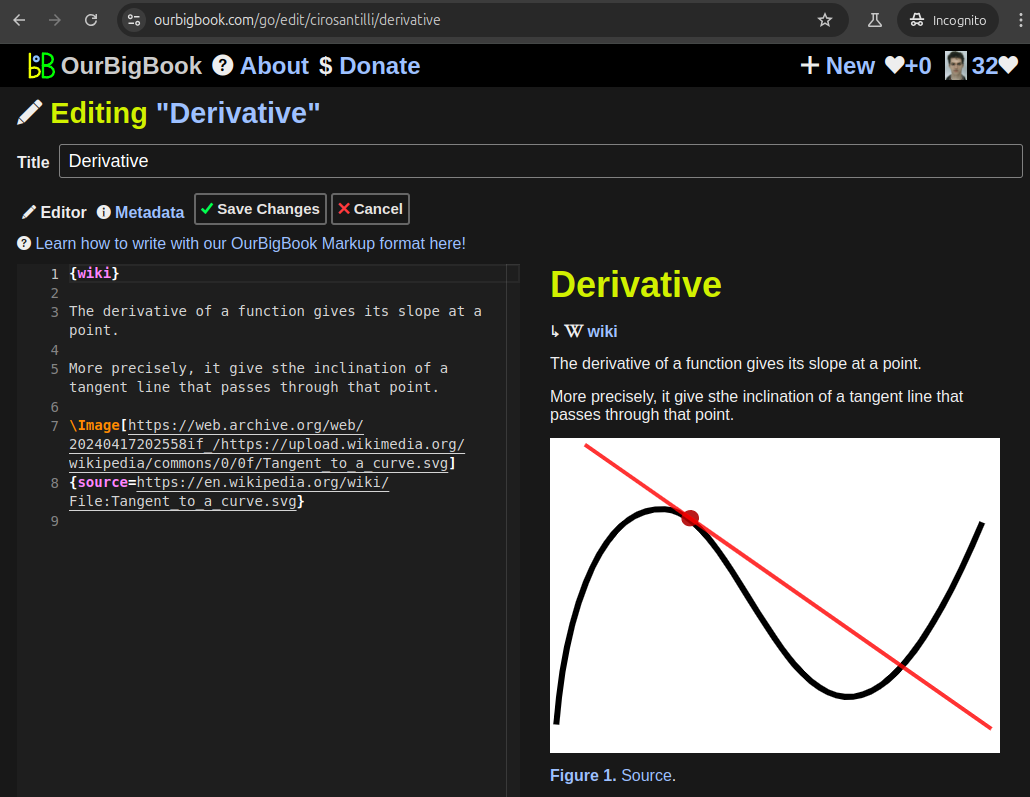
Figure 5. . You can also edit articles on the Web editor without installing anything locally. Video 3. Edit locally and publish demo. Source. This shows editing OurBigBook Markup and publishing it using the Visual Studio Code extension. 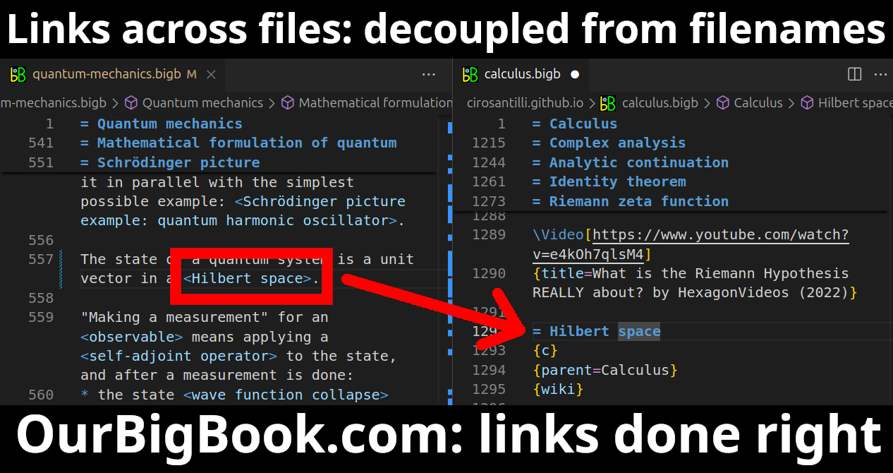
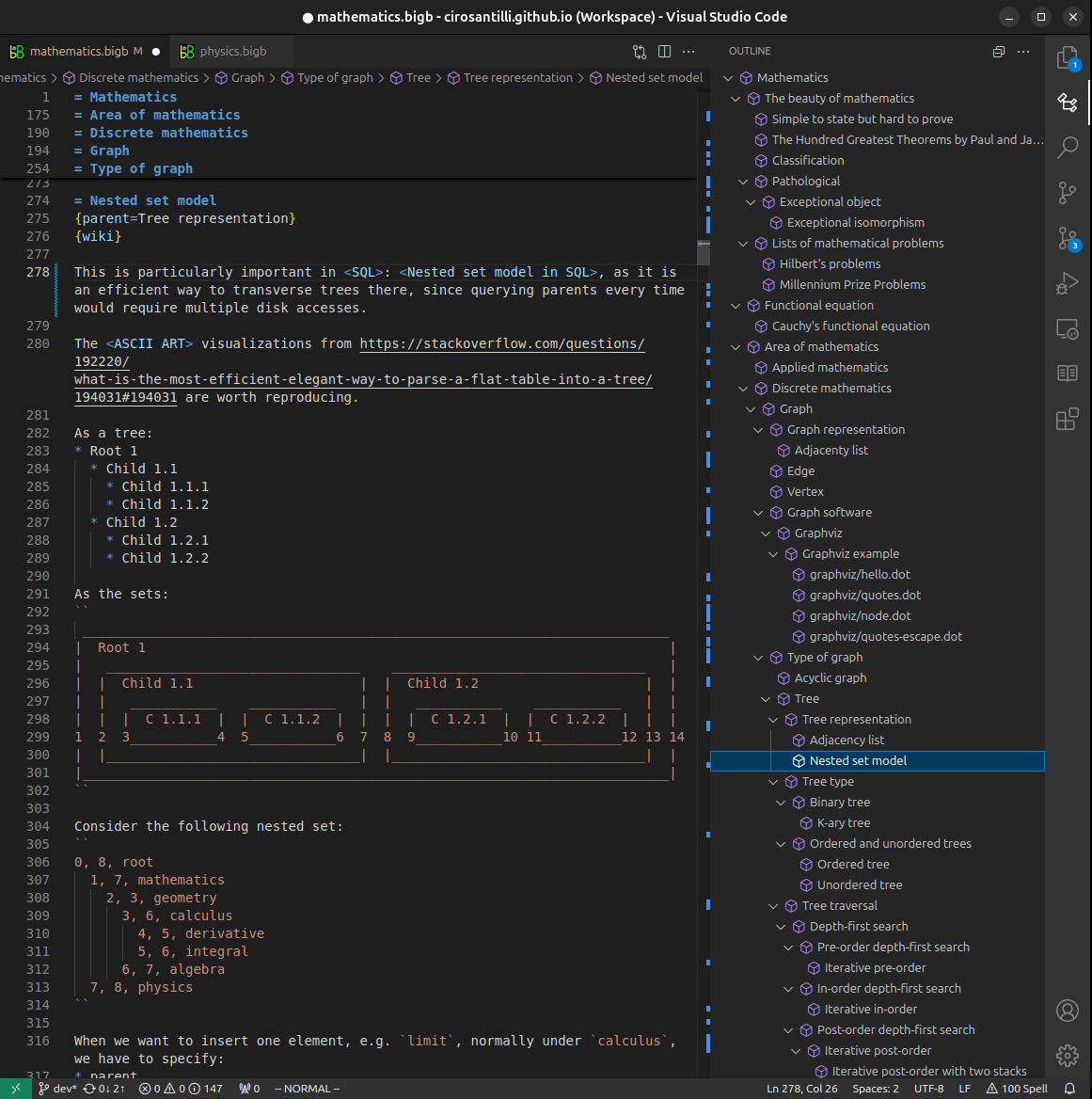
- Infinitely deep tables of contents:


All our software is open source and hosted at: github.com/ourbigbook/ourbigbook
Further documentation can be found at: docs.ourbigbook.com
Feel free to reach our to us for any help or suggestions: docs.ourbigbook.com/#contact