Rosemary Candlin might refer to a specific individual or concept, but there isn't widespread information about a figure or topic by that name. It's possible that she could be a person known in a specific context, such as academia, art, literature, or another field that has not gained significant public attention.
Sharon Glotzer is a prominent physicist known for her work in the fields of condensed matter physics and materials science. She is particularly recognized for her research on the behavior of complex fluids, soft materials, and the theoretical frameworks that describe their properties. Glotzer has made significant contributions to understanding the self-assembly of nanoparticles and the design of new materials at the nanoscale.
Ted Belytschko is a prominent figure in the field of computational mechanics and engineering, recognized for his contributions to the development of numerical methods and algorithms for analyzing complex materials and structures. He has been involved in advancing techniques such as the finite element method and meshfree methods, which are used for simulating physical phenomena in various engineering applications, including solid and fluid mechanics. Belytschko has also contributed significantly to the fields of computational biology and materials science.
EcosimPro is a simulation software platform designed for modeling and simulating complex systems in various fields such as engineering, environmental studies, and complex systems. It provides tools for dynamic modeling, enabling users to create detailed simulations of systems involving physical, chemical, biological, and economic processes. The software is particularly useful for applications in areas like: 1. **Energy systems**: Modeling power generation, distribution, and consumption.
Goma is a distributed compiler infrastructure developed by Google. It is designed to speed up the compilation of source code by distributing the compilation tasks across multiple machines. Goma allows developers to leverage the power of multiple CPUs, reducing the overall build time in large codebases, which is particularly beneficial for projects that involve a significant amount of code compilation.
As of my last knowledge update in October 2023, "SaltMod" refers to a mod for the game "Dwarf Fortress." The "SaltMod" is a modification that brings various enhancements, new features, and changes to the gameplay experience in Dwarf Fortress, which is known for its complex simulation and management mechanics.
"Visualizing Energy Resources Dynamically on the Earth" generally refers to the use of visualization techniques and tools to represent and analyze energy resources across the globe in a dynamic manner. This can include various forms of data related to energy resources such as solar, wind, fossil fuels, hydroelectric power, and geothermal energy. The dynamic aspect often implies the use of real-time or regularly updated data, enabling users to observe changes over time.
EdDSA, or Ed25519, is a digital signature scheme that is part of the EdDSA (Edwards-Curve Digital Signature Algorithm) family. It was designed to be secure, efficient, and easy to implement. EdDSA is based on elliptic curve cryptography and utilizes the Edwards curve.
Java KeyStore (JKS) is a secure storage mechanism in Java used for managing cryptographic keys, certificates, and trusted certificate authorities (CAs). It is part of the Java Security framework and provides a way to protect key material in a binary format that can be easily managed by Java applications.
As of my last update in October 2023, the Open Vote Network is an initiative designed to promote transparency and accessibility in voting systems, often using blockchain or other decentralized technologies. The goal of the Open Vote Network is to ensure that electoral processes are verifiable, tamper-proof, and accessible to a wider audience, enabling individuals to verify their votes and ensure fair election outcomes.
Signcryption is a cryptographic primitive that combines the functionality of digital signatures and encryption into a single process. It allows a sender to simultaneously encrypt a message and generate a signature for that message in a way that is more efficient than performing each operation separately. ### Key Features of Signcryption: 1. **Efficiency**: Signcryption typically reduces the computational resources and time required for both signing and encrypting a message, making it a more efficient alternative to separately signing and then encrypting a message.
Locksmithing is the art and science of designing, making, and repairing locks and security devices. It involves a variety of skills and knowledge, including: 1. **Lock Design and Fabrication**: Creating and manufacturing locks, considering mechanics and security features. 2. **Key Cutting and Design**: Crafting keys to fit specific locks, including duplicating existing keys and creating unique keys for new locks.
Dynamic Intelligent Currency Encryption (DICE) is a security framework designed to protect digital transactions and currency exchanges, particularly in the realm of cryptocurrencies and online financial transactions. While specific details can vary, the general concepts associated with DICE revolve around enhancing the security and integrity of financial data through advanced encryption methodologies.
Casualism, in philosophy, refers to a perspective that emphasizes the role of causation in understanding phenomena, particularly in the realms of metaphysics, epistemology, and ethics. While the term may not always be uniformly defined, it generally revolves around the idea that events, actions, and states of affairs can be understood primarily in terms of their causal relationships. In metaphysics, casualism might focus on how causation constructs reality and how entities or phenomena are interconnected through causal chains.
Ground Sample Distance (GSD) is a measurement used in remote sensing, photogrammetry, and mapping that indicates the distance between two consecutive pixel centers on the ground, expressed in units such as centimeters or meters. It reflects the level of detail that can be resolved in an aerial image or satellite image.
The VisionMap A3 is a high-resolution digital mapping system designed for aerial photogrammetry. It combines advanced hardware and software technologies to capture detailed aerial imagery and create accurate geographic data. This system is particularly useful for topographic mapping, geographic information systems (GIS), land-use planning, and other applications requiring precise spatial information. Key features of the VisionMap A3 system typically include: 1. **High Resolution:** The system can capture high-resolution images that are suitable for various mapping applications.
The concept of a **visual hull** is primarily associated with computer vision and graphics, particularly in the context of 3D reconstruction and modeling from multiple 2D images or views. A visual hull can be understood as follows: - **Definition**: The visual hull of an object is the intersection of the visual cones from multiple viewpoints. In simpler terms, it represents the volume within which an object must lie, based on the silhouettes or outlines captured in images from different angles.
A pansharpened image is a type of satellite or aerial imagery that combines high-resolution panchromatic imagery with lower-resolution multispectral imagery to create a single image that maintains the fine spatial details from the panchromatic image while preserving the color information from the multispectral bands. ### Key Components: 1. **Panchromatic Image**: This is a single-band image that captures a broad range of wavelengths, usually in the visible spectrum. It has a higher spatial resolution (i.e.
Multispectral imaging is a technique that captures image data at specific frequency ranges across the electromagnetic spectrum. Unlike traditional imaging that typically uses only visible light, multispectral imaging collects data across multiple wavelengths, including ultraviolet, visible, and infrared light. The key features of multispectral imaging include: 1. **Multiple Wavelengths**: Multispectral cameras capture data from several discrete bands, usually ranging from 3 to 10 different wavelengths, though some systems may capture more.
Satellite imagery of North Korea refers to the use of satellite technology to capture images of the Earth's surface, particularly focused on the Korean Peninsula. These images can provide valuable insights into various aspects of the country, such as its geography, infrastructure, military installations, agricultural land, and urban development.
Pinned article: Introduction to the OurBigBook Project
Welcome to the OurBigBook Project! Our goal is to create the perfect publishing platform for STEM subjects, and get university-level students to write the best free STEM tutorials ever.
Everyone is welcome to create an account and play with the site: ourbigbook.com/go/register. We belive that students themselves can write amazing tutorials, but teachers are welcome too. You can write about anything you want, it doesn't have to be STEM or even educational. Silly test content is very welcome and you won't be penalized in any way. Just keep it legal!
Intro to OurBigBook
. Source. We have two killer features:
- topics: topics group articles by different users with the same title, e.g. here is the topic for the "Fundamental Theorem of Calculus" ourbigbook.com/go/topic/fundamental-theorem-of-calculusArticles of different users are sorted by upvote within each article page. This feature is a bit like:
- a Wikipedia where each user can have their own version of each article
- a Q&A website like Stack Overflow, where multiple people can give their views on a given topic, and the best ones are sorted by upvote. Except you don't need to wait for someone to ask first, and any topic goes, no matter how narrow or broad
This feature makes it possible for readers to find better explanations of any topic created by other writers. And it allows writers to create an explanation in a place that readers might actually find it.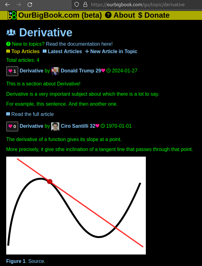
Figure 1. Screenshot of the "Derivative" topic page. View it live at: ourbigbook.com/go/topic/derivativeVideo 2. OurBigBook Web topics demo. Source. - local editing: you can store all your personal knowledge base content locally in a plaintext markup format that can be edited locally and published either:This way you can be sure that even if OurBigBook.com were to go down one day (which we have no plans to do as it is quite cheap to host!), your content will still be perfectly readable as a static site.
- to OurBigBook.com to get awesome multi-user features like topics and likes
- as HTML files to a static website, which you can host yourself for free on many external providers like GitHub Pages, and remain in full control
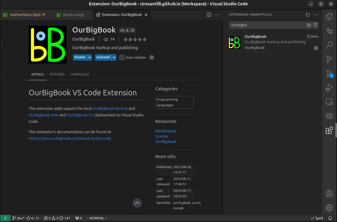
Figure 3. Visual Studio Code extension installation.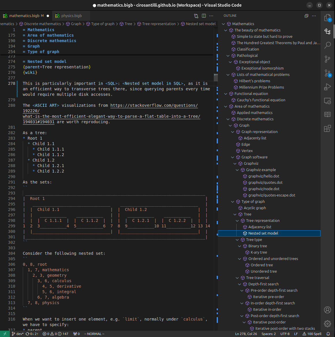
Figure 4. Visual Studio Code extension tree navigation.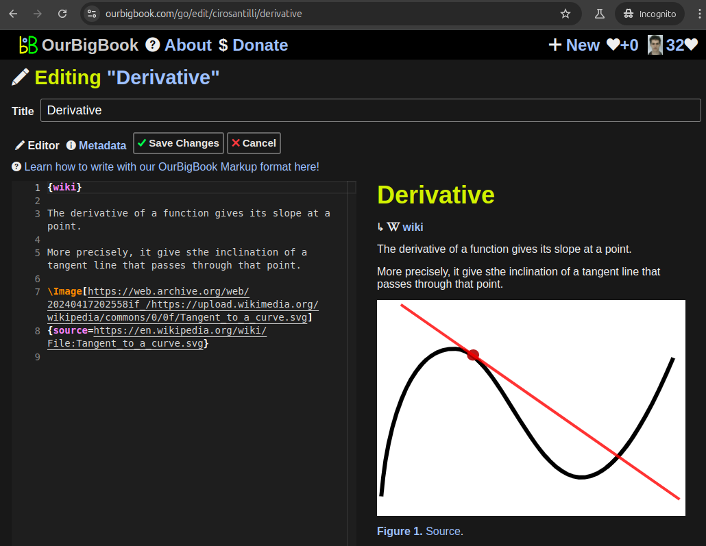
Figure 5. Web editor. You can also edit articles on the Web editor without installing anything locally.Video 3. Edit locally and publish demo. Source. This shows editing OurBigBook Markup and publishing it using the Visual Studio Code extension.Video 4. OurBigBook Visual Studio Code extension editing and navigation demo. Source. 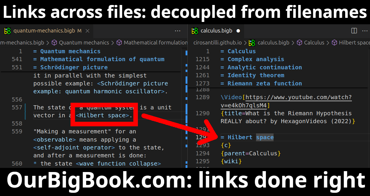
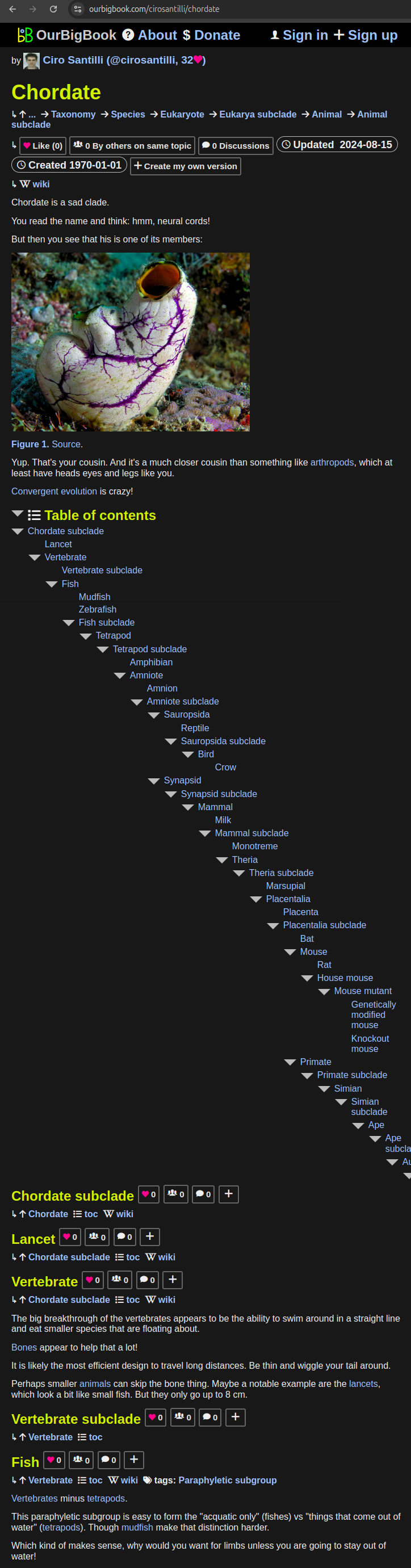
- Infinitely deep tables of contents:

All our software is open source and hosted at: github.com/ourbigbook/ourbigbook
Further documentation can be found at: docs.ourbigbook.com
Feel free to reach our to us for any help or suggestions: docs.ourbigbook.com/#contact