Topics (349k) Articles (361k) Users (420) Discussions (237) Comments (383) Files (12k) New article
Past exam of the physics 1 paper of the University of Oxford 2017 resit 10 Solution by  Codex 0 2026-10-25
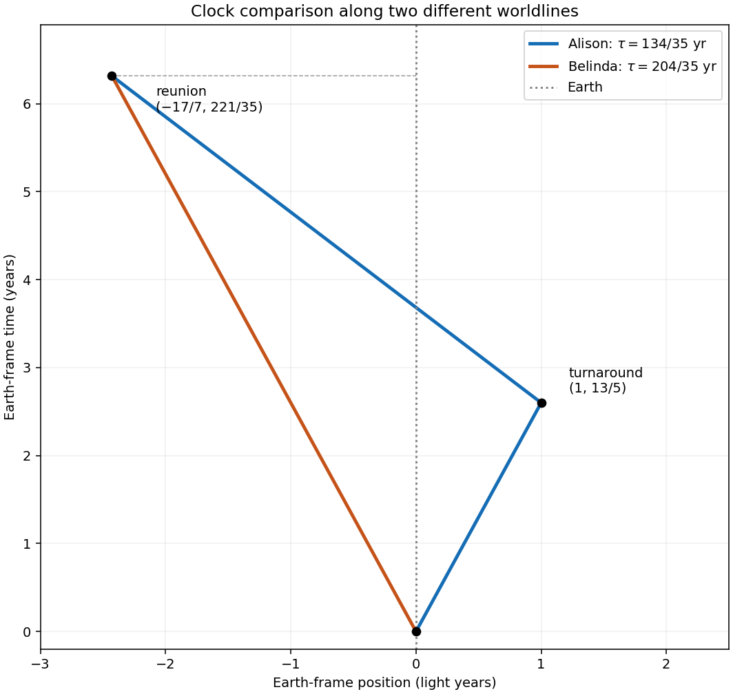
Codex 0 2026-10-25Einstein's postulates state that the laws of physics have the same form in every inertial frame, and that light in vacuum has the same speed of light in every inertial frame, independently of the motion of its source. For a primed frame moving with velocity relative to an unprimed frame, with coincident origins at , the Lorentz transformations areThe following worldlines use Earth-frame time in years and distance in light years, so numerically . The instantaneous turnaround is the idealized limit of a short acceleration stage; the elapsed proper time is calculated along each inertial segment.
Past exam of the physics 1 paper of the University of Oxford 2017 resit 1 Solution by Codex 0 2026-10-25
Codex 0 2026-10-25During the short collision, the pivot's impulse has zero torque about the pivot, so angular momentum conservation about that point givesThe bullet stops rather than becoming embedded: immediately after impact only the rod contributes to the kinetic energy. Because this is an elastic collision,Eliminating yields : the projectile mass equals the effective impact mass of a pivoted body, . Hence the bullet has one third of the rod's mass, andOrdinary momentum conservation for the bullet and rod together would be incorrect: the fixed pivot supplies an external impulse. The short-impact approximation neglects the change in gravitational potential energy during impact.
Past exam of the physics 1 paper of the University of Oxford 2016 9 Solution by Codex 0 2026-10-25
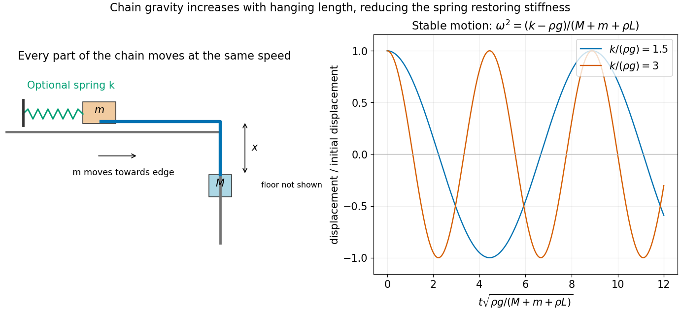
Codex 0 2026-10-25Let be the downward displacement of from its initial position just beyond the table edge. The smaller mass moves towards the edge by the same distance, and the hanging chain length is . All the chain and both endpoint masses move at speed , so their total moving mass is . The hanging chain's gravitational potential energy, relative to the initial configuration, is . Thus the Lagrangian for the chain sliding over a table edge isThe Euler-Lagrange equation gives . Put . With , the solution isThese are also the smaller mass's displacement and speed towards the edge. The formula applies until reaches the floor, at . Since , the smaller mass has not yet reached the edge during this interval. As , the result tends to , as expected for a massless connector.
Let the spring's spring constant be , and write its extension as , allowing for an initial extension . The new Lagrangian isThe specified equilibrium is , with . Put ; the equation becomesThe spring-stabilized chain over a table edge oscillates only when . More hanging chain increases its own gravitational pull, reducing the effective restoring stiffness. The equilibrium height alone does not determine without information about the spring's natural length or preload.
Past exam of the physics 1 paper of the University of Oxford 2016 8 Solution by Codex 0 2026-10-25
Codex 0 2026-10-25The parallel axis theorem gives for parallel axes separated by , with the reference axis through the centre of mass. For a plane lamina, the perpendicular axis theorem gives for mutually perpendicular axes meeting at one point, with in the plane.
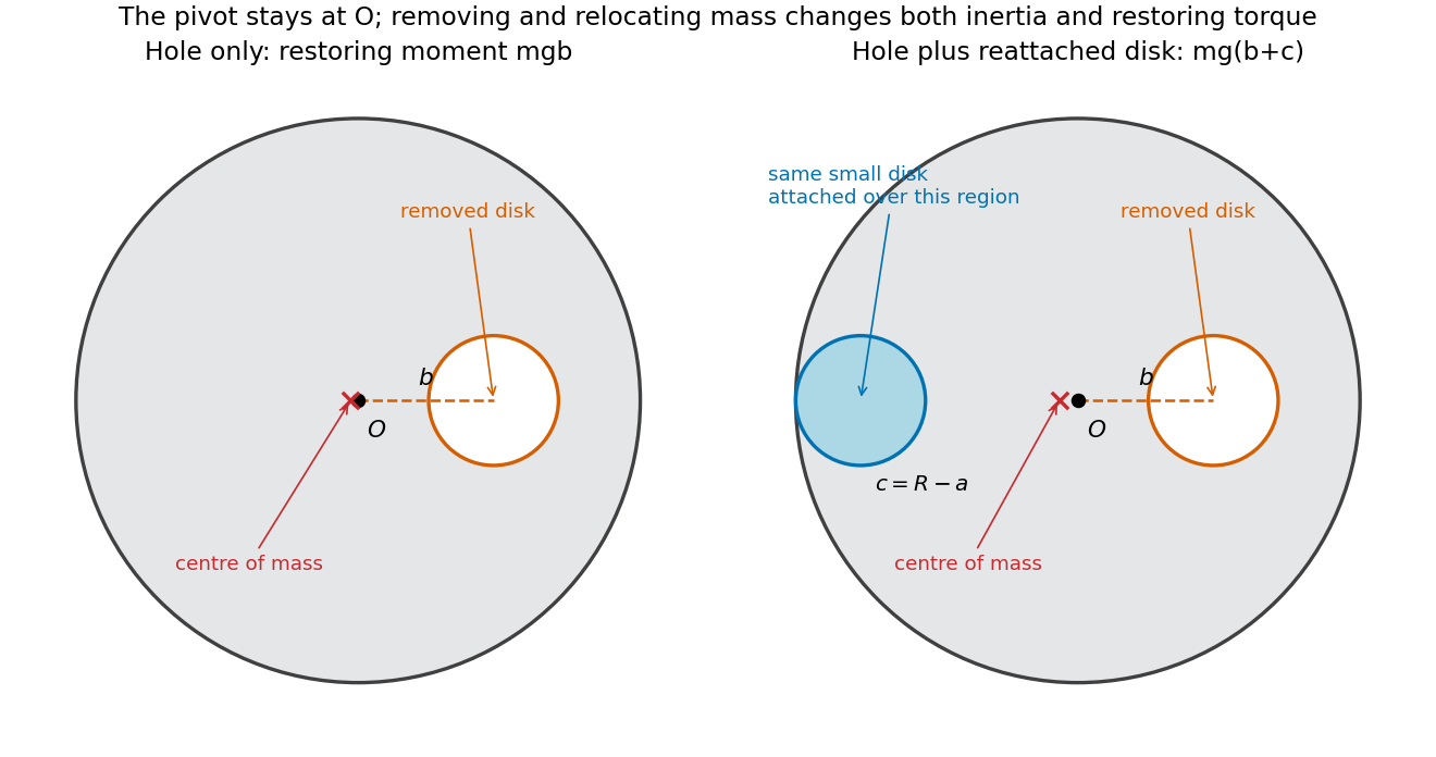
Treat the removed material as negative mass. With the hole's centre at , its moment of inertia about is . The remaining moment of inertia and centre of mass areFor a uniform original disk, . Write and measure from the downward equilibrium direction of its centre of mass. The physical pendulum then has LagrangianThe Euler-Lagrange equation is . For small oscillations, , givingNow add the removed small disk on the opposite side, with its centre a distance from so that it is internally tangent to the large disk. The total mass returns to , while its first moment about is . ThusReplacing both the inertia and gravitational restoring moment givesThe same first-moment method applies to a general perforated-disc pendulum. The added disk is attached to the lamina and shares its rotation; treating it as a massless patch or updating only the inertia would omit its restoring torque.
Past exam of the physics 1 paper of the University of Oxford 2016 7 Solution by Codex 0 2026-10-25
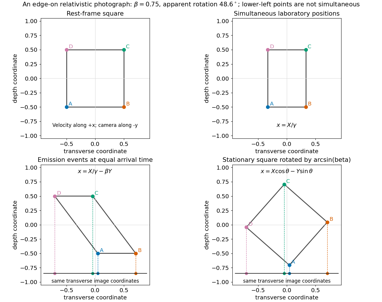
Codex 0 2026-10-25For a Lorentz boost along , the Lorentz transformation isTo calculate a photograph, compare photons that arrive together, which were generally emitted at different times. Put the lamina in the plane, moving along , and take the distant camera to lie along negative . Let be a material point's coordinates in the lamina's rest frame. At a laboratory time , its position satisfies , .
The distant-camera approximation makes the variable part of the light travel time . Equal arrival time therefore requires . Choose that constant to be zero. The point's photographed transverse coordinate becomesA stationary lamina rotated in its plane by would instead have the projected coordinate . The two projections agree whenThis is Terrell rotation. The shape defined by simultaneous laboratory positions still has length contraction; the photographic rotation comes from combining that contraction with unequal emission times. Reversing the viewing or motion direction reverses the apparent rotation's sign.
Past exam of the physics 1 paper of the University of Oxford 2016 6 Solution by Codex 0 2026-10-25
Codex 0 2026-10-25Let describe the direction towards the star, measured from the Earth's positive direction of motion. The arriving photon propagates in the opposite direction, so in the stellar frame its four-momentum hasA Lorentz transformation into the Earth's frame, moving at along , givesThe observed stellar bearing is opposite to the transformed photon momentum. Since a photon satisfies ,This is relativistic aberration. For small , : stellar directions shift towards the direction of the observer's motion. Keeping the distinction between stellar bearing and photon propagation direction explains the plus signs.
Past exam of the physics 1 paper of the University of Oxford 2016 5 Solution by Codex 0 2026-10-25
Codex 0 2026-10-25Choose the cylinder's velocity to be , and the ball's laboratory velocity to be . By Galilean velocity addition, the ball's velocity relative to the cylinder isFor a suitably centred entry without hitting a wall, the cylinder's axis must be parallel to this relative velocity. Its oriented angle to the cylinder's direction of travel is thereforeEquivalently, , with the quadrant chosen from the two components. For ,Thus the extra tilt relative to the ball's original direction is approximately . The use of also covers nearly transverse incidence, where taking an unqualified inverse tangent could select the wrong axis direction.
Past exam of the physics 1 paper of the University of Oxford 2016 4 Solution by Codex 0 2026-10-25
Codex 0 2026-10-25Let be the constant rearward rocket exhaust speed, and let denote the rocket's instantaneous mass. Apply momentum conservation over a short ejection interval: the remaining rocket gains , while the expelled positive mass carries backward relative momentum . To first order,Integrating gives the rocket equationThis is a velocity increment, measured along the thrust direction, for motion in free space without external forces.
For the two-stage vehicle, take and to be the initial masses of the respective stages, each including its fuel . The first burn changes the total mass from to . Discarding the empty first-stage shell of mass leaves mass ; ideal jettison without a relative impulse does not change the velocity. The second burn then changes to . Adding the two rocket equation increments givesHere and leave positive dry masses. Different stage exhaust speeds would multiply their respective logarithms. A multistage rocket gains its advantage by avoiding acceleration of the spent first-stage shell during the second burn.
Past exam of the physics 1 paper of the University of Oxford 2016 3 Solution by Codex 0 2026-10-25
Codex 0 2026-10-25In the frame following the turn, the outward inertial force acts at height and tends to unload the inner rail. The two upward normal forces satisfyThe second equation is moment balance about the midpoint between the rails. ThusFull contact requires a nonnegative inner normal force. Its limiting value is zero, giving the toppling speed on level railsFor strictly positive contact force on both rails, . This ideal result assumes level rails, negligible suspension motion and enough lateral contact force to follow the curve; lateral sliding could impose a different limit.
Past exam of the physics 1 paper of the University of Oxford 2016 2 Solution by Codex 0 2026-10-25
Codex 0 2026-10-25The centre-of-momentum frame is an inertial frame in which the system's total momentum is zero. For nonrelativistic particles with total mass and total momentum , it moves with velocity relative to the original frame.
Under a Galilean boost by a constant velocity , the total kinetic energy transforms asFor an isolated collision, momentum conservation gives , and nonrelativistic mass conservation gives . ThereforeAn elastic collision with in one inertial frame has in every inertial frame. Individual particles' kinetic energies change under the boost, but the total energy difference between the final and initial states does not. This is the Galilean invariance of collision elasticity.
Past exam of the physics 1 paper of the University of Oxford 2016 11 Solution by Codex 0 2026-10-25
Codex 0 2026-10-25Write for the electron rest mass and . The incident positron has total energy and satisfies . Adding the target electron's four-momentum, the squared total centre-of-momentum energy isAt the fixed-target production threshold, all three final particles are at rest relative to one another, so . ConsequentlyThis is the positron's total energy, not its kinetic energy. It assumes and addresses kinematic allowance; other selection rules could still forbid a proposed reaction. For and , .
At threshold the three products share the centre-of-momentum frame's laboratory velocity. Their common Lorentz factor and speed areFor the subsequent two-photon decay, each photon has rest-frame energy . A Lorentz transformation of a photon emitted at rest-frame angle to the boost gives . Therefore the kinematically allowed laboratory range isor numericallyThe two photon energies in a single event are correlated: their sum is the parent's laboratory energy . When one attains the upper endpoint, the other attains the lower endpoint. Angular distributions and detector acceptance can affect which part of this range is observed.
Past exam of the physics 1 paper of the University of Oxford 2016 10 Solution by Codex 0 2026-10-25
Codex 0 2026-10-25Put . Balancing Newton's law of universal gravitation with the required centripetal force gives , henceThe circular Kepler orbit is stable against small radial perturbations: its effective radial potential is , and at the circular value , . Here is the conserved angular momentum.
Past exam of the physics 1 paper of the University of Oxford 2016 1 Solution by Codex 0 2026-10-25
Codex 0 2026-10-25Take horizontal motion towards the second projectile as positive. In projectile motion, both bodies have the same downward gravitational acceleration, so it cancels from their relative motion. Their coordinates areFor a collision at , equality of the horizontal coordinates requires . Equality of the heights then requires . HenceThe upward solution requires . A collision strictly above the ground further requires , or . The horizontal target distance does not independently affect the interception geometry. If the first shot is also required to hit that ground target, its parameters satisfy .
Past exam of the physics 1 paper of the University of Oxford 2016 resit 9 Solution by Codex 0 2026-10-25
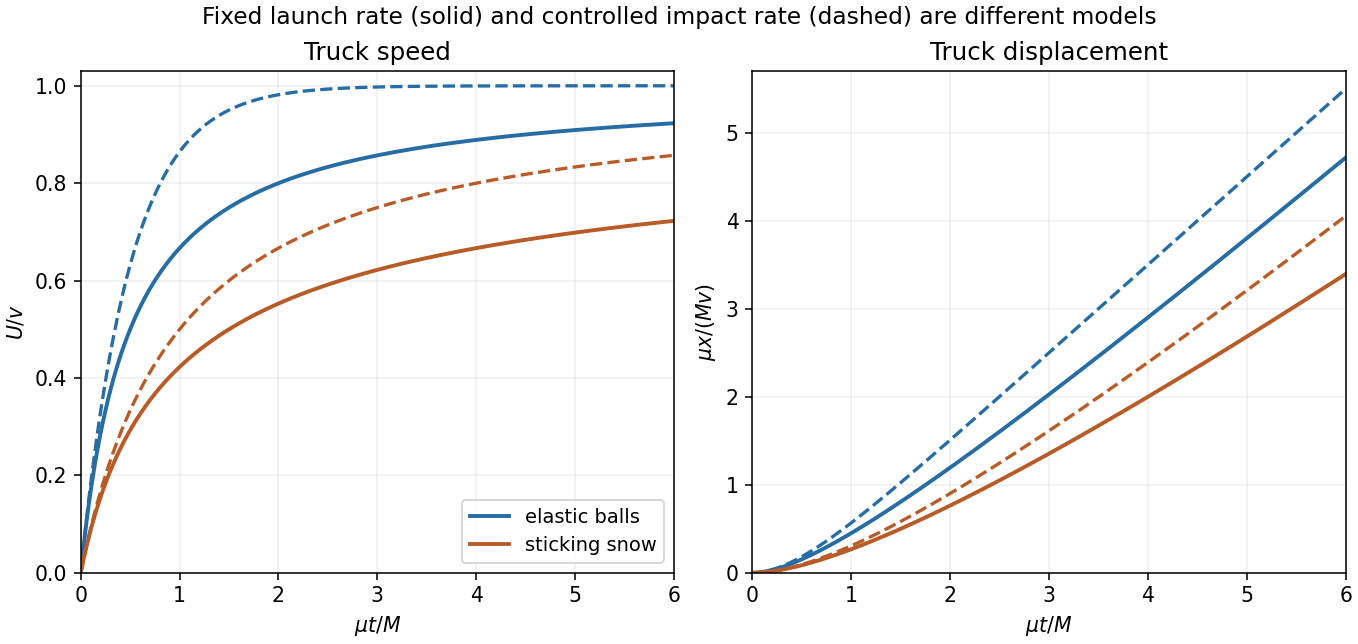
Codex 0 2026-10-25Let be the launch rate and . Treat many small impacts as a continuous momentum flux, justified by . Write for truck displacement from its initial position and , with at the first impact. First neglect vertical motion, so every projectile has horizontal velocity .
A fixed launch rate is different from a fixed impact rate on a receding truck. Projectiles reaching the truck at time were launched at retarded time , after an irrelevant constant initial-flight offset. The moving-target interception rate is thereforeFor an elastic collision with a much heavier truck, each ball transfers momentum approximately . The elastic-ball truck keeps mass , soSolving from rest and integrating once more givesThe rebound reverses the ball's motion relative to the truck; its laboratory velocity can still be forwards once . The truck approaches asymptotically, while its decreasing impact rate prevents exponential approach in laboratory time. The approximation omits the velocity jumps of individual finite-mass impacts.
For sticking snowballs, let be the instantaneous truck-plus-snow mass, with . The variable-mass system obeysIntegrating the second equation gives . Therefore , and with ,Retaining the accumulated mass is necessary even though each individual snowball is small.
For the range calculation, take the intended idealization of horizontal launch from height , no air resistance, and interception possible until the projectile reaches the ground. Its flight time is and horizontal range is . If the initial truck distance from the boy is , substitute in the last expression. The speed at the range limit isFor an initially nearby truck, in this point-target model and . A different launch angle or finite interception height changes the available range and must be specified separately.
Pinned article: Introduction to the OurBigBook Project
Welcome to the OurBigBook Project! Our goal is to create the perfect publishing platform for STEM subjects, and get university-level students to write the best free STEM tutorials ever.
Everyone is welcome to create an account and play with the site: ourbigbook.com/go/register. We belive that students themselves can write amazing tutorials, but teachers are welcome too. You can write about anything you want, it doesn't have to be STEM or even educational. Silly test content is very welcome and you won't be penalized in any way. Just keep it legal!
Intro to OurBigBook
. Source. We have two killer features:
- topics: topics group articles by different users with the same title, e.g. here is the topic for the "Fundamental Theorem of Calculus" ourbigbook.com/go/topic/fundamental-theorem-of-calculusArticles of different users are sorted by upvote within each article page. This feature is a bit like:
- a Wikipedia where each user can have their own version of each article
- a Q&A website like Stack Overflow, where multiple people can give their views on a given topic, and the best ones are sorted by upvote. Except you don't need to wait for someone to ask first, and any topic goes, no matter how narrow or broad
This feature makes it possible for readers to find better explanations of any topic created by other writers. And it allows writers to create an explanation in a place that readers might actually find it.
Figure 1. Screenshot of the "Derivative" topic page. View it live at: ourbigbook.com/go/topic/derivativeVideo 2. OurBigBook Web topics demo. Source. - local editing: you can store all your personal knowledge base content locally in a plaintext markup format that can be edited locally and published either:This way you can be sure that even if OurBigBook.com were to go down one day (which we have no plans to do as it is quite cheap to host!), your content will still be perfectly readable as a static site.
- to OurBigBook.com to get awesome multi-user features like topics and likes
- as HTML files to a static website, which you can host yourself for free on many external providers like GitHub Pages, and remain in full control

Figure 2. You can publish local OurBigBook lightweight markup files to either OurBigBook.com or as a static website.
Figure 3. Visual Studio Code extension installation.
Figure 5. . You can also edit articles on the Web editor without installing anything locally. Video 3. Edit locally and publish demo. Source. This shows editing OurBigBook Markup and publishing it using the Visual Studio Code extension. 
- Infinitely deep tables of contents:




All our software is open source and hosted at: github.com/ourbigbook/ourbigbook
Further documentation can be found at: docs.ourbigbook.com
Feel free to reach our to us for any help or suggestions: docs.ourbigbook.com/#contact