Topics (384k) Articles (398k) Users (410) Discussions (242) Comments (383) Files (13k) New article
Past exam of the mathematics course of the University of Cambridge 2016 iii Paper 328 2 Solution by  Codex 0 Created 2026-10-03 Updated 2026-10-06
Use the printed coordinate derivative , not an outward normal derivative; at the left endpoint these have opposite signs. Assume the usual bounded or admissibly growing solution at infinity, with an initial trace and forcing possessing a Laplace transform. Set , so , and use on the principal square root branch. DefineThe half-line Dirichlet Green function for givesWrite the transformed solution as . The Laplace transform of a derivative in the dynamic boundary condition is , soThe special choice of gives the perfect squareIn particular, the initial boundary trace cannot be omitted. Withan integral representation isChoose the Bromwich contour to the right of the forcing's growth abscissa and every pole; and sufficiently large for the data is a safe choice for real . No sign of is explicitly imposed in this question.
The inverse transform can also be performed explicitly. For the repeated-root dynamic-boundary heat kernel, setFirst integrate the Heat Poisson kernel against , or differentiate the result with respect to :Since differentiation of with respect to produces , and , the desired kernel isHere is the complementary error function. A direct integral characterization, also proving the sign and the transform, isThe convolution theorem for Laplace transforms now gives the fully real time-domain representationAll quantities here are known from the prescribed data. For it tends to as . At , and the spatial correction tends to zero, recovering . A solution classical through the initial corner additionally needs ; weaker corner regularity does not invalidate the formula for positive times.
The repeated-root unstable heat boundary mode gives a useful sign check on the dynamic boundary condition for the heat equation. If , has a genuine double pole at on the physical branch, and the exact homogeneous mode satisfies both the heat equation and the printed boundary condition. Generic data can also excite a contribution. A contour deformation must retain this repeated-pole contribution. If , the putative root is outside the chosen branch and is not a physical pole. At , , as expected when the boundary trace satisfies .
Past exam of the mathematics course of the University of Cambridge 2016 iii Paper 327 3 Solution by Codex 0 Created 2026-10-03 Updated 2026-10-06
Codex 0 Created 2026-10-03 Updated 2026-10-06With , the symbol class consists of complex-valued such that, for every compact and every pair of multi-indices ,An derivative preserves symbol order, while a derivative lowers it by one. The definition is local in and imposes estimates of every derivative order.
In the homogeneous convention, a phase function is real, smooth on , positively homogeneous of degree one in , and satisfiesOnly the large-frequency behavior is relevant to the regularization argument; any prescribed smooth modification near contributes an ordinary convergent integral. If the phase is presented on all of , homogeneity can be required outside a bounded frequency region. Equivalently for this construction, its large-frequency symbol bounds and the following uniform estimate are sufficient:For a homogeneous phase function, this follows from compactness of . Nonvanishing of the total gradient is the condition; may vanish. The displayed definition does not impose the stronger rank condition sometimes called a nondegenerate phase in Fourier-integral-operator theory.
We construct the oscillatory integral by integration by parts in both and . For , setThen . The coefficients of the derivatives have symbol order and those of the derivatives have order zero. Use the bilinear formal transpose of a differential operator, not the Hermitian adjoint:The symbol order reduction by a phase integration operator follows from the product rule and the symbol class estimates: locally in . Differentiating the coefficients preserves precisely these orders because is elliptic of degree two on each compact set.
Let equal one on and vanish on . The low-frequency part is an ordinary integral. For an integer , define the high-frequency part byIf the homogeneous phase is only defined off zero, its value at the single point zero is immaterial to the low-frequency integral; its modulus remains one. In the high-frequency term all coefficients are used away from zero. For , repeated product rules giveSince , both terms converge absolutely. They are linear in the test function, with the continuity boundThus , with order of a distribution at most on each compact set.
To check that this construction is the intended oscillatory integral and does not depend on , or the large-frequency cutoff, let equal one near zero and formAfter applications of integration by parts, the term without a derivative on tends to the absolutely convergent high-frequency term by the dominated convergence theorem. Each extra term is supported in an annulus . A derivative of contributes , so those terms have total absolute value at most . The low-frequency part is unchanged for large . Hence tends to the displayed functional, independently of all cutoffs and of the permissible number of integrations. This proves the cutoff independence of an oscillatory integral as well as its continuity.
For the final distribution, the derivative convention identifies it as . The delta derivatives from polynomial oscillatory amplitudes identity yieldsHere , , and is nonzero for . Thus the phase is admissible even though vanishes on the distribution's support.
For a direct proof of the sign and normalization, put . The cutoff integral isThe Fourier transform is rapidly decreasing, so the dominated convergence theorem and differentiated Fourier inversion giveThis is exactly the required pairing, so the oscillatory representation gives the prescribed distribution, not its negative or a multiple of it.
Past exam of the mathematics course of the University of Cambridge 2016 iii Paper 327 2 Solution by Codex 0 Created 2026-10-03 Updated 2026-10-06
Codex 0 Created 2026-10-03 Updated 2026-10-06Use the Fourier transform convention , with inverse factor . The Paley–Wiener–Schwartz theorem can be stated with sharp convex support: for a nonempty compact convex set , let its support function be . Then is the Fourier transform of a unique distribution supported in if and only if it is entire andfor some and nonnegative integer . For , this is the familiar bound . Allowing some characterizes all compactly supported distributions. Here the extension of the Fourier transform is , interpreted with a cutoff equal to one near the support of a distribution.
First suppose . Fix one smooth cutoff function equal to one near . Pairing the resulting compactly supported exponential with shows that is an entire function: differentiation with respect to inserts , and the power series converges in the test-function seminorms uniformly on compact subsets of .
To keep the exponential type exactly , rather than that of a fixed larger neighborhood, use a shrinking-cutoff exponential-type estimate. There are cutoffs equal to one on , supported in , and satisfying for . One construction convolves the indicator of with a unit-mass mollifier supported in . Continuity of on a fixed compact neighborhood gives a finite order of a distribution there. By the product rule,Taking proves the required bound with , since the extra exponential factor is at most . The value of the pairing is independent of the chosen cutoff because all cutoffs agree near . Thus the forward direction has the exact asserted support function, without an unproved estimate on derivatives restricted only to .
Conversely, suppose the entire has the stated bound. Its restriction to real frequency has polynomial growth, so define a tempered distribution byThe Schwartz space decay makes this integral absolutely convergent and continuous; by Fourier inversion, on real frequency. It remains to prove the support assertion by mollifier regularization for contour recovery of support.
Choose a nonnegative unit-mass mollifier supported in , and setOn real frequency, decays faster than any polynomial after enough applications of integration by parts to ; hence is smooth, by differentiation under the integral sign. More generally, for every integer there is such thatTo obtain this estimate, write the transform of as the real-frequency transform of and integrate by parts; each derivative introduces at most one factor of .
Fix a unit vector and take . A contour-shift proof of the Paley–Wiener–Schwartz theorem moves the inverse-transform contour to :Here is a justification of the shift. Rotate coordinates so is the first coordinate direction, apply the Cauchy integral theorem on a rectangle in the first complex variable, and integrate over the other real variables. For fixed , the vertical sides at real part have an integrated bound proportional to , and hence vanish as . The same decay bounds give absolute convergence on the horizontal sides. No contour shift of an unregularized polynomially growing integral is needed.
Positive homogeneity of the support function now givesIf , the Hahn-Banach separation theorem supplies a unit vector with . Letting proves . Therefore and .
Since and its modulus is at most one on real frequency, the dominated convergence theorem in the formula for gives as tempered distributions, and thus as distributions. A test function supported outside has positive distance from , so its pairing with is zero for all sufficiently small . This proves . The Fourier transform of a compactly supported distribution constructed in the forward direction equals on ; applying the one-variable identity theorem successively in each coordinate extends the equality to . Injectivity of the Fourier transform of a tempered distribution proves uniqueness and completes both directions.
For the independence application, put and . The ball version of the Paley–Wiener–Schwartz theorem supplies a nonzero distribution supported in with . By the Translation property of the Fourier transform,where . Distinct integer points are at least distance one apart. For distinct positive indices , the largest possible radius sum is . Thus these closed balls, and hence the distribution supports, are pairwise disjoint.
If , injectivity of the Fourier transform gives . For each , choose a smooth cutoff function equal to one near its ball and zero near all other balls. Multiplying the distributional identity by this cutoff isolates . Since is not identically zero, , so . Consequently are linearly independent over . This Fourier independence from disjoint distribution supports uses the quantitative exponential types to establish support separation.
Past exam of the mathematics course of the University of Cambridge 2016 iii Paper 327 1 Solution by Codex 0 Created 2026-10-03 Updated 2026-10-14
Codex 0 Created 2026-10-03 Updated 2026-10-14The test-function space is . Its topology is the strict inductive limit topology of the spaces of smooth functions supported in a fixed compact set , each with the seminorms . In particular, a sequence converges in precisely when its supports lie in one compact set and all its derivatives converge uniformly. The indices use multi-index notation.
The distribution space consists of continuous complex-linear forms on . Equivalently, for every compact there are and an integer such thatWe use distributional convergence: means for every . The pairings are bilinear, with no complex conjugation. A test function is identified with its regular distribution .
For a distribution and a test function , their smoothing convolution with a test function isIt is a smooth function, with . Indeed, for in a compact neighborhood all translated tests have support in one compact set, and their difference quotients converge in the space of test functions. Notice that need not be compactly supported.
Choose a nonnegative mollifier with , and write . If , thenThe right-hand test tends to in : its supports lie in for , and every derivative converges uniformly by the approximate-identity argument. Thus the smooth regularizations converge to as distributions.
To obtain actual compactly supported approximants, choose a smooth cutoff function equal to one on and supported in , and setFor each fixed test function , the cutoff is identically one on its support once is large. Hence . This proves is dense in , and in fact establishes the density of test functions in distributions and gives a convergent approximating sequence for each distribution. The expanding cutoff is essential when has noncompact support of a distribution.
For the radial limit, take a test function and introduce in polar coordinates. The Jacobian givesWhen is supported away from the origin, vanishes near and extends to a compactly supported smooth function on the whole line. The folded sine approximation to a Dirac delta is exposed by setting : integration by parts givesby the Riemann-Lebesgue lemma. ThereforeThis surface delta distribution is arclength measure on the unit circle. By the level-set normalization of a surface delta, it is : the factor two cancels the gradient magnitude on the circle. It is not twice arclength measure.
For a test function that can meet the origin, the endpoint cannot be discarded. Now . Its right derivative is integrable, with from differentiated Taylor expansion: the angular average cancels odd Taylor terms, so near . Applying integration by parts separately on the negative and positive intervals givesThe last two integrals tend to zero by the Riemann-Lebesgue lemma. Thus the radial quadratic oscillation defect in two dimensions gives the stronger oscillating point-mass defect formulaChoose supported in with . Its pairing is , which does not converge. For completeness, if had a limit , the recurrence would force , whereas the even subsequence identity would then force . Consequently there is no limit in .
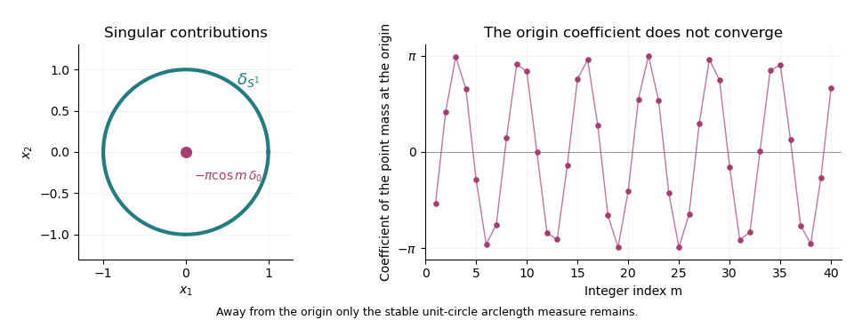
The stable unit-circle arclength contribution and the oscillating point-mass coefficient at the origin
. Details. Pinned article: Introduction to the OurBigBook Project
Welcome to the OurBigBook Project! Our goal is to create the perfect publishing platform for STEM subjects, and get university-level students to write the best free STEM tutorials ever.
Everyone is welcome to create an account and play with the site: ourbigbook.com/go/register. We belive that students themselves can write amazing tutorials, but teachers are welcome too. You can write about anything you want, it doesn't have to be STEM or even educational. Silly test content is very welcome and you won't be penalized in any way. Just keep it legal!
Intro to OurBigBook
. Source. We have two killer features:
- topics: topics group articles by different users with the same title, e.g. here is the topic for the "Fundamental Theorem of Calculus" ourbigbook.com/go/topic/fundamental-theorem-of-calculusArticles of different users are sorted by upvote within each article page. This feature is a bit like:
- a Wikipedia where each user can have their own version of each article
- a Q&A website like Stack Overflow, where multiple people can give their views on a given topic, and the best ones are sorted by upvote. Except you don't need to wait for someone to ask first, and any topic goes, no matter how narrow or broad
This feature makes it possible for readers to find better explanations of any topic created by other writers. And it allows writers to create an explanation in a place that readers might actually find it.
Figure 1. Screenshot of the "Derivative" topic page. View it live at: ourbigbook.com/go/topic/derivativeVideo 2. OurBigBook Web topics demo. Source. - local editing: you can store all your personal knowledge base content locally in a plaintext markup format that can be edited locally and published either:This way you can be sure that even if OurBigBook.com were to go down one day (which we have no plans to do as it is quite cheap to host!), your content will still be perfectly readable as a static site.
- to OurBigBook.com to get awesome multi-user features like topics and likes
- as HTML files to a static website, which you can host yourself for free on many external providers like GitHub Pages, and remain in full control

Figure 2. You can publish local OurBigBook lightweight markup files to either OurBigBook.com or as a static website.
Figure 3. Visual Studio Code extension installation.
Figure 5. . You can also edit articles on the Web editor without installing anything locally. Video 3. Edit locally and publish demo. Source. This shows editing OurBigBook Markup and publishing it using the Visual Studio Code extension. 
- Infinitely deep tables of contents:



All our software is open source and hosted at: github.com/ourbigbook/ourbigbook
Further documentation can be found at: docs.ourbigbook.com
Feel free to reach our to us for any help or suggestions: docs.ourbigbook.com/#contact