 Continuation predictor-corrector step

For the cubic polynomial, an oriented, normalized tangent vector isIts Euclidean norm is one and $DF(z_k)t_k=0$. The sign here follows increasing $x$; for a general solution branch, choose the sign of each new tangent vector so its dot product with the previous one is positive. First predict $z_{\mathrm{p}}=z_k+h{t}_k$, then apply Newton method starting at $z_{\mathrm{p}}$ toThe second equation keeps the correction on the transverse line in this two-dimensional example; in higher dimensions it is a hyperplane. Solving the linear system $DH(z^{(j)})\delta z=-H(z^{(j)})$ and updating $z^{(j+1)}=z^{(j)}+\delta z$ corrects both coordinates together.

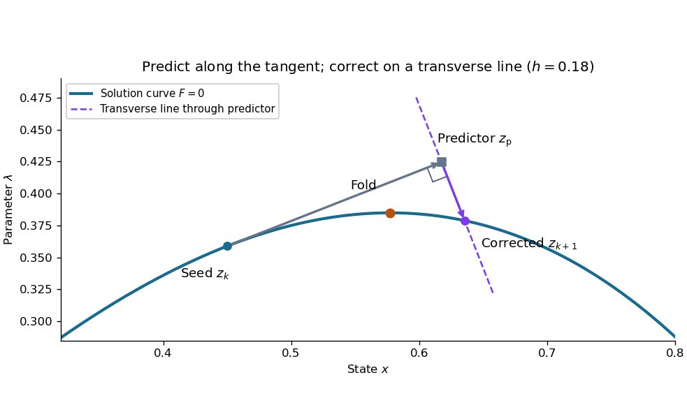
This step gives $z_{\mathrm{p}}\approx (0.617556,0.424641)$ and $z_{k+1}\approx (0.635532,0.378840)$. Check both equations: the solution must satisfy $x^3-x+\lambda =0$ and $t_k^{\mathsf{T}}(z-z_{\mathrm{p}})=0$. Checking only the first could accept any point on the solution branch. The new $x$ exceeds $1/\sqrt{3}$, so the step crosses the continuation fold, even though the predictor's $\lambda$ exceeds $2/(3\sqrt{3})$.

At the seed, set $a=3x_k^2-1$. The determinant of the correction Jacobian matrix with the exact unit vector above isAt either continuation fold, $a=0$, $t_k=(1,0)$ and $DH(z_k)=\left(\begin{array}{cc}0& 1\\ 1& 0\end{array}\right)$: the correction remains invertible. More generally, if $DF$ has full rank and a one-dimensional kernel spanned by $t_k$, adding $t_k^{\mathsf{T}}$ gives an invertible matrix, since a vector annihilated by both rows must be zero. This is a local argument; the old transverse hyperplane need not work arbitrarily far along the curve. Reduce $h$ and retry when correction fails, and check the equations and orientation after successful steps. Scaling state and parameter coordinates also matters, because it changes the Euclidean norm used to normalize the tangent vector.

// Target: analysis.bigb