Discrete Fourier transform
ID: discrete-fourier-transform

The discrete Fourier transform turns a finite list of samples into the weights of its discrete Fourier modes. The goal is to reveal a simple oscillatory recipe hidden in complicated-looking data, while retaining enough information to reconstruct every sample exactly. In signal processing, those weights identify sampled frequencies and wave phases; in numerical analysis, they simplify circular convolution and the discrete sine transform Poisson solver.
Start with eight real samples, indexed by :Writing , the actual list isThe discrete Fourier transform recovers the recipe asThe constant contributes ; the cosine contributes ; the half-sized sine contributes and . All other coefficients vanish exactly. The imaginary coefficients carry the sine's wave phase, which a plot of absolute values alone would hide.
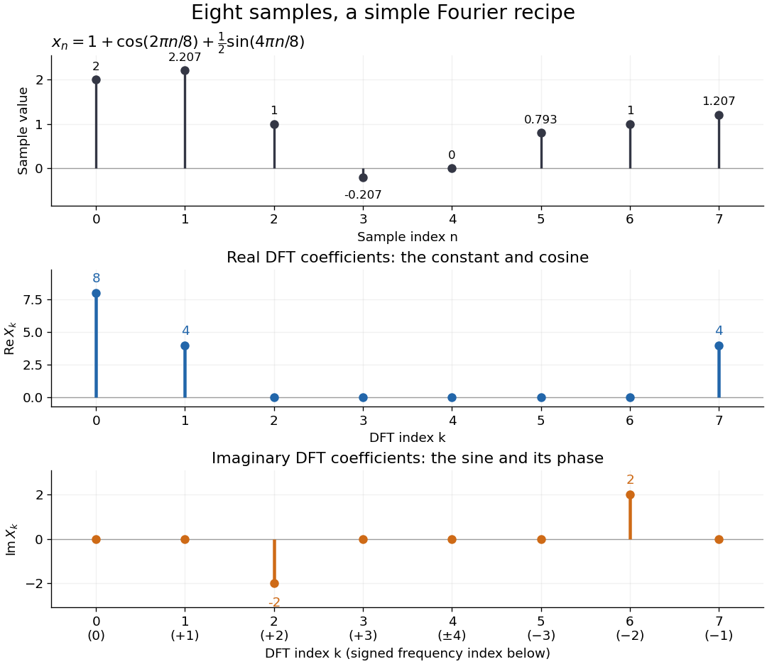
Precisely, for a positive integer and a vector , the forward discrete Fourier transform and inverse discrete Fourier transform used here areThus the forward exponent has a minus sign and no scale factor; the inverse exponent has a plus sign and the factor . The coefficients in the reconstruction are , rather than . In the example, , the pair reconstructs the cosine, and the pair reconstructs the half-sized sine. These conventions agree with the scaled Fourier coefficients in MIT's authored notes.[ref]
https://ocw.mit.edu/courses/6-02-introduction-to-eecs-ii-digital-communication-systems-fall-2012/06d7972059805d20e6a7db3a52ec23f2_MIT6_02F12_chap13.pdf. Hari Balakrishnan, Christopher Terman, and George Verghese, MIT 6.02 notes, Chapter 13, equations (13.15)–(13.16), 2012
The proof idea is orthogonality of roots of unity: for integers ,Distinct discrete Fourier modes cancel in this finite geometric series. Substituting the forward formula into the inverse discrete Fourier transform leaves only the desired sample. The same orthogonality makes the normalized discrete Fourier modes an orthonormal basis and gives the discrete Parseval identity, in the present convention,For the eight-sample example, direct squaring gives , while , so . This identity preserves the squared L2 norm after accounting for normalization. The existing discrete Parseval identity instead scales the forward discrete Fourier transform by , producing a unitary matrix and equal squared L2 norms without the factor .
For real input, discrete Fourier conjugate symmetry pairs positive and negative frequencies. The label is a residue modulo : when represents the same discrete Fourier mode as , since . It therefore represents negative frequency cycles per sample. If samples are seconds apart, the corresponding signed frequency is cycles per second. Similarly, index represents , while index is its own negative modulo .
The discrete Fourier transform is an invertible map between two finite vectors. The continuous Fourier transform instead describes a function on the real line by an integral over a continuous frequency variable. A finite list of samples does not determine the full continuous frequency spectrum: aliasing of discrete Fourier modes already supplies distinct waveforms with identical observations. Applying the inverse formula at arbitrary integer indices gives the periodic extension of a finite sequence, repeating the recorded block every samples. This is a property of that representation, rather than evidence that the physical signal repeats beyond the recording. Laurent Demanet's MIT notes place the discrete Fourier transform alongside the continuous Fourier transform and Fourier series to explain the role of sampling and repetition.[ref]
https://math.mit.edu/icg/resources/teaching/18.330/18.330-Mar21.pdf. Laurent Demanet, Introduction to Numerical Analysis, MIT 18.330, §§6.2–6.3, pp. 57–60, March 22, 2012
The beauty is that a change of basis exposes cancellation and structure without losing data. Direct evaluation needs sums of terms; a Fast Fourier transform computes the same discrete Fourier transform with far less work. Computational speed and the mathematical meaning of the coefficients are separate questions.

The Discrete Fourier Transform (DFT) is a mathematical technique used to analyze the frequency content of discrete signals. It expresses a finite sequence of equally spaced samples of a function in terms of its frequency components. The DFT converts a sequence of time-domain samples into a sequence of frequency-domain representations, allowing us to examine how much of each frequency is present in the original signal.


Output: another sequence of complex numbers such that:Intuitively, this means that we are braking up the complex signal into sinusoidal frequencies:and is the amplitude of each sine.
- : is kind of magic and ends up being a constant added to the signal because
- : sinusoidal that completes one cycle over the signal. The larger the , the larger the resolution of that sinusoidal. But it completes one cycle regardless.
- : sinusoidal that completes two cycles over the signal
- ...
- : sinusoidal that completes cycles over the signal
Motivation: similar to the Fourier transform:In particular, the discrete Fourier transform is used in signal processing after a analog-to-digital converter. Digital signal processing historically likely grew more and more over analog processing as digital processors got faster and faster as it gives more flexibility in algorithm design.
- compression: a sine would use N points in the time domain, but in the frequency domain just one, so we can throw the rest away. A sum of two sines, only two. So if your signal has periodicity, in general you can compress it with the transform
- noise removal: many systems add noise only at certain frequencies, which are hopefully different from the main frequencies of the actual signal. By doing the transform, we can remove those frequencies to attain a better signal-to-noise
Sample software implementations:
- numpy.fft, notably see the example: numpy/fft.py
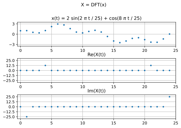
DFT of with 25 points
. This is a simple example of a discrete Fourier transform for a real input signal. It illustrates how the DFT takes N complex numbers as input, and produces N complex numbers as output. It also illustrates how the discrete Fourier transform of a real signal is symmetric around the center point. New to topics? Read the docs here!