 Kernel density estimation

Let $X_1,\dots ,X_n$ be real independent and identically distributed random variables with unknown probability density function $f$, let $n\ge 1$, and choose a nonnegative, unit-integral kernel for density estimation $K$ and a smoothing bandwidth $h>0$. The kernel density estimator isPlace a bump at every observation and add their contributions. Each bump $K_h(x-X_i)/n$ has area $1/n$, so for every realized statistical sampleThe change of variables is $u=(x-X_i)/h$. Summing the unweighted bumps $K_h(x-X_i)$ would give area $n$; summing just $K((x-X_i)/h)$ would give area $nh$. Those raw sums do not have the normalization of a probability density function.

Unlike a histogram, the construction does not require choosing bin origins, and a Gaussian density kernel gives a smooth curve. Its appeal is that identical local contributions can combine into a probability density function with several peaks without first choosing their number. This makes kernel density estimation useful for exploring an unknown probability distribution and estimating interval probabilities, while the smoothing bandwidth controls how much detail is visible.

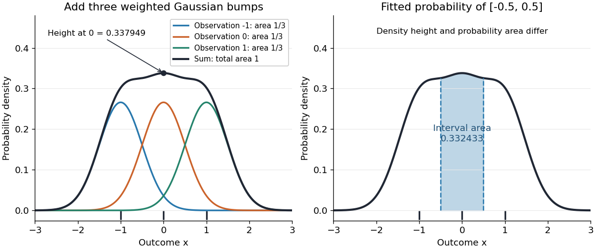
Before the statistical sample is observed, ${\hat{f}}_{n,h,K}$ is a random function; afterwards it is a fitted probability density function. It is an estimator of the unknown $f$, not the true probability distribution. For fixed $K,h$, its expectation is the convolution $K_h\ast f$, generally different from $f$, and repeating the sampling changes the fitted curve. The exact mean integrated squared error of a kernel density estimator separates this smoothing bias of an estimator from sampling variance. Allowing signed kernels of order ell retains the formula but can lose nonnegativity.