Orthogonal polynomial
ID: orthogonal-polynomial

An orthogonal polynomial family chooses polynomials that do not overlap under a specified inner product. For real polynomials on an interval , use the weighted inner productAssume , the weight is measurable and positive almost everywhere, and its absolute moments are finite for every integer . These conditions make the integrals finite and give every nonzero polynomial positive squared norm. A sequence is an orthogonal polynomial family when has real coefficients and polynomial degree exactly , and for .[ref]
18 Orthogonal Polynomials. NIST Digital Library of Mathematical Functions; Koornwinder, Wong, Koekoek, Swarttouw and Reinhardt, NIST DLMF Chapter 18, §18.2(i), equations 18.2.1 and 18.2.1_5: interval orthogonality and finite absolute moments
Here and is the Kronecker delta. Orthogonality does not require : an orthonormal set is obtained only after replacing by . Multiplying each member by any nonzero real constant preserves orthogonality, but changes its norm and the corresponding expansion coefficient. The monic orthogonal polynomial convention instead fixes each leading coefficient to one.
The first four Legendre polynomials, named for Adrien-Marie Legendre, use on and the normalization :Their orthogonality and squared norms areThus their Gram matrix has a positive diagonal and zero entries elsewhere, although their function graphs cross and overlap on the page. Orthogonality measures an integral of products, rather than separation of function graphs.[ref]
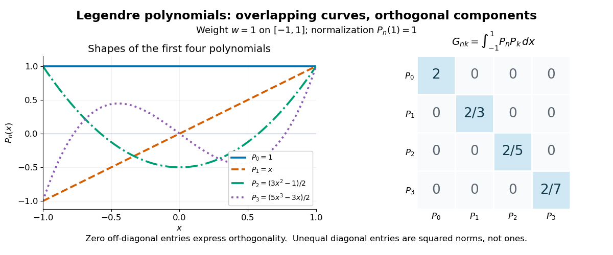
The first four Legendre polynomials and their exact integral Gram matrix: orthogonal, with unequal squared norms
. Details. 
For these four polynomials, a short verification expands each product and uses and . For example, and . The same calculation gives the diagonal entries . More generally, apply the Gram-Schmidt process to the monomial basis : at step , subtract projections onto the earlier polynomials. The result retains its leading term, has degree , and has positive norm, proving existence without a differential equation. Different degrees also give linear independence, so form a basis of the polynomials of degree at most .
This basis turns least-squares solutions for functions into independent scalar calculations, as the decoupled coefficients of orthogonal polynomial projections show. In a spectral method, increasing the degree enlarges the approximation space while keeping earlier projection coefficients fixed. Weighted integrals also connect the same orthogonal polynomials to Gaussian quadrature: its nodes are polynomial roots of a member of the family. The projection problem minimizes an integrated squared error; Gaussian quadrature uses the family to choose evaluation points for an integral.
New to topics? Read the docs here!