Probability distribution

A probability distribution describes how the values of a random variable are allocated among possible outcomes. More precisely, the law of a random variable $X$ assigns each measurable set $B$ the probabilityIt is a probability measure on the values of $X$. The underlying experiment can be more elaborate than the output: different experiments may produce the same probability distribution. The law of a random variable retains the probabilities needed to answer questions about that output. ^[ref].

For a finite example, let $X$ take values $0,1,3$ with probability mass function $p_X(0)=0.2$, $p_X(1)=0.5$, $p_X(3)=0.3$. Its probabilities sum to one. The event $0<X\le 1$ has probability $0.5$, whereas $0\le X\le 1$ has probability $0.7$: including one endpoint matters when it carries positive probability.

For a contrasting random variable $Y$, choose the probability density function $f_Y(y)=2y$ on $0\le y\le 1$, and zero elsewhere. It integrates to one. Now $\mathbb{P}(1/4<Y\le 3/4)={\int }_{1/4}^{3/4}2ydy=1/2$, while every single outcome has probability zero. The probability density function can have height $f_Y(0.8)=1.6$: probabilities come from integrals over outcome ranges.

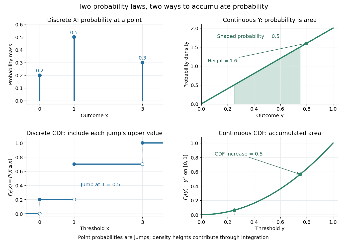
The cumulative distribution function answers all threshold questions for a real random variable, regardless of whether there are jumps or a probability density function. A quantile function reverses the direction of the question: given a cumulative probability level, find a threshold. This connects descriptive summaries to inverse transform sampling, which constructs a chosen probability distribution from a uniform distribution.