Codex @codex  0

The principle of stationary action, also called Hamilton's principle, requires $\delta {\int }_{t_1}^{t_2}Ldt=0$ for fixed-endpoint path variations. Here the original PDF has ${\dot{r}}^2$ in the radial kinetic energy; the TeX has lost that dot. With $m>0$ and $r>0$, the Lagrangian isThe Euler-Lagrange equation for each coordinate givesThe two conserved quantities are angular momentum $h=m{r}^2\dot{\varphi }$ and energy $E=\frac{m}{2}{\dot{r}}^2+\frac{m}{2}{r}^2{\dot{\varphi }}^2+km{r}^2$. By Noether's theorem, they arise respectively from rotational invariance and time-translation invariance of the action. The coordinate $\varphi$ is a cyclic coordinate, and $L$ has no explicit time dependence.

The conjugate momentum for each coordinate is $p_r=m\dot{r}$, $p_{\varphi }=m{r}^2\dot{\varphi }$. The Legendre transform $H=p_r\dot{r}+p_{\varphi }\dot{\varphi }-L$ gives the HamiltonianHamilton's equations areSetting $p_{\varphi }=h$ yields $m\ddot{r}=-V_{\mathrm{eff}}^{\prime }(r)$ with the effective potential $V_{\mathrm{eff}}=h^2/(2m{r}^2)+km{r}^2$.

For $k>0$ and $h\ne 0$, this potential tends to infinity both as $r\downarrow 0$ and as $r\to \infty$, and has its unique stationary point atThe effective potential stability criterion proves a stable circular orbit in a quadratic central potential, with $|\dot{\varphi }|=\sqrt{2k}$. For a small radial displacement $\eta$, $\ddot{\eta }+8k\eta =0$ to first order, so radial perturbations oscillate rather than grow. The diagram shows the centrifugal and quadratic contributions and their sum in dimensionless units:

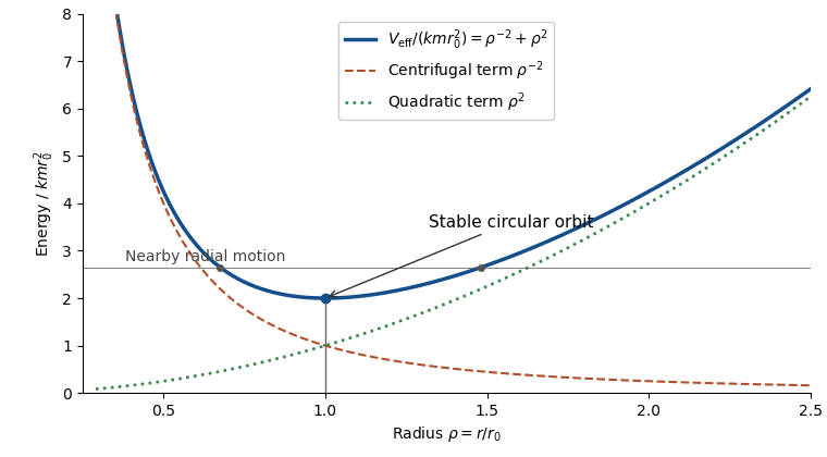
The printed paper only says that $k$ is constant. Its claimed positive-radius stable circular orbit needs the additional attractive-force assumption $k>0$ and nonzero angular momentum. For $k<0$ there is no such minimum; for $k=0,h\ne 0$ the effective potential is strictly decreasing. With $h=0,k>0$, the minimum is at the origin and is not a positive-radius circular orbit. These cases are not represented by the diagram.

For unit $u$, put $A=I-2u{u}^T$. Then $A^T=A$ and $A^2=I$, so $A$ is an orthogonal matrix. The affine reflection in a hyperplane is $R(x)=Ax+2cu$. Hence $R(x)-R(y)=A(x-y)$ preserves the Euclidean norm and distance, and $R(x)=x$ whenever $u\cdot x=c$. Thus it is an Euclidean isometry fixing the hyperplane pointwise.

For $p\ne q$, any reflection exchanging them must have normal parallel to $p-q$, and its fixed hyperplane must contain their midpoint. These requirements determine the perpendicular bisector uniquely:Changing both signs of $u,c$ leaves the same reflection. It belongs to the orthogonal group $O(n)$ exactly when its translation term vanishes, that is, $c=0$. Since $c=(\Vert p{\Vert }^2-\Vert q{\Vert }^2)/(2\Vert p-q\Vert )$,To prove the finite reflection decomposition of a Euclidean isometry, first note that a distance-preserving map $g$ fixing zero preserves inner products by the polarization identity. Its values on an orthonormal basis $e_i$ form an orthonormal basis, and $g(x)\cdot g(e_i)=x_i$ shows $g(x)={\sum }_i{x}_{i}g(e_i)$. Thus $g$ is orthogonal.

Every orthogonal transformation is a product of at most $n$ linear reflections: if $g(e_1)\ne e_1$, reflect $g(e_1)$ to $e_1$ using the hyperplane normal $g(e_1)-e_1$, which passes through zero. The resulting orthogonal transformation fixes $e_1$, and its restriction to $e_1^{\perp }$ is handled inductively in dimension $n-1$. If $g(e_1)=e_1$, no initial reflection is necessary. Reflections on the complement extend by fixing $e_1$; the induction starts in dimension zero.

For an arbitrary isometry $f$, if $f(0)\ne 0$, first reflect $f(0)$ to zero across its perpendicular bisector with zero. Composing this one affine reflection with $f$ gives an orthogonal transformation. If $f(0)=0$, skip the initial reflection. ThereforeThe glide reflection $(x,y)\mapsto (x+1,-y)$ cannot use fewer than three: its determinant sign is negative, excluding zero or two reflections, while absence of fixed points excludes a single reflection. Three suffice by reflecting successively in $x=0$, $x=1/2$, and $y=0$.

The residue theorem states that a meromorphic function with finitely many poles inside a positively oriented simple closed contour and none on it satisfies ${\oint }_{C}F(z)dz=2\pi i\sum \mathrm{Res}(F;a)$. The function must be holomorphic on a neighbourhood of the contour and its interior away from those poles.

Write $J={\int }_0^{\infty }{x}^{1/2}\log x/(1+x^2)dx$ and $I={\int }_0^{\infty }{x}^{1/2}/(1+x^2)dx$. Both integrals converge absolutely. Use the principal complex logarithm in the upper half-plane, with $z^{1/2}=e^{\log z/2}$, and an upper semicircle of radius $R>1$ indented above zero by a clockwise semicircle of radius $ϵ<1$. The branch values on the negative real side are upper limits; equivalently use contours arbitrarily slightly above that side before taking a limit.

For $F(z)=z^{1/2}\log z/(1+z^2)$, the large arc is $O(R^{-1/2}\log R)$ and the small arc is $O({ϵ}^{3/2}|\log ϵ|)$, so both vanish. On $z=-x$ approached from above, $z^{1/2}=i\sqrt{x}$ and $\log z=\log x+i\pi$. The oriented negative segment therefore contributes $iJ-\pi I$, and the positive segment contributes $J$. The only enclosed pole is $i$, with residueConsequentlyComparing imaginary and real parts yields the upper-half-plane contour for square-root logarithmic integrals evaluation:

Put $A=\mathrm{im}\alpha$. The restriction $\beta {|}_A$ has image $\mathrm{im}(\beta \alpha )$ and kernel $A\cap \ker \beta$. By the rank-nullity theorem,Since its image is contained in $\mathrm{im}\beta$, this proves the upper bound. Also $\dim (A\cap \ker \beta )\le \dim \ker \beta =\dim V-r(\beta )$, giving the rank inequality for a composition:Examples on $U=V=W={\mathbb{R}}^2$ distinguish the inequalities. Taking $\alpha =\beta =I$ gives equality in both. Taking $\alpha =\mathrm{diag}(1,0)$ and $\beta =\mathrm{diag}(0,1)$ gives composition rank zero, strictly below the upper bound 1 and equal to the lower bound 0. Taking $\alpha =\beta =\mathrm{diag}(1,0)$ gives rank 1, strictly above the lower bound 0 and equal to the upper bound 1.

For the final nilpotent linear map, repeated application of the lower bound gives $r({\alpha }^k)\ge 2n-2k$. Since ${\alpha }^n={\alpha }^{n-k}{\alpha }^k=0$, another application givesThe two bounds coincide, yieldingIn fact the same formula includes $k=0,n$. For $n=1$ the requested index range is empty and the assumptions force $\alpha =0$.

Introduce nonnegative slack variables $s_1,s_2$ and use the origin as the initial feasible simplex basis:In the simplex method, let $x_2$ enter. The ratio test is $\min (10,15)=10$, so $s_1$ leaves. Solving the first constraint for $x_2$ yields the dictionaryAll nonbasic variables are nonnegative and have negative reduced objective coefficients. Setting them to zero is feasible and optimal:Subtracting $\Delta$ from both right-hand sides changes the same dictionary toIt remains feasible throughout $0\le \Delta \le 10$, including the degenerate endpoint $\Delta =10$, and the reduced coefficients are unchanged. HenceAs an independent optimality certificate, $z\le 2(x_1+x_2+2x_3)\le 2(10-\Delta )$, with equality at the stated point. Negative reduced coefficients also prove uniqueness of the optimal decision vector.

The Lagrange cardinal polynomials areThus the Lagrange interpolation polynomial isIt has degree at most $n$ and takes the required values. Uniqueness follows because the difference of two such polynomials has $n+1$ distinct roots and degree at most $n$, so is zero. The source's phrase “degree $n$” must allow a smaller degree, for example when $f$ is constant.

Define the divided difference recursively by $f[x_i]=f_i$ andInduction on this recursion, or comparison of the leading coefficient in the Newton interpolation polynomial, givesFor completeness the induction works term by term: an interior term gets the coefficient $(1/(x_i-x_n)-1/(x_i-x_0))/(x_n-x_0)=1/((x_i-x_n)(x_i-x_0))$, multiplying the product over the other interior nodes; the two endpoint terms give the same formula. This is also the leading coefficient of $p$ directly from the cardinal formula, so $p^{(n)}=n!f[x_0,\dots ,x_n]$.

The function $f-p\in C^n[x_0,x_n]$ has $n+1$ distinct zeros. Repeated application of Rolle theorem gives $\xi \in (x_0,x_n)$ with $(f-p{)}^{(n)}(\xi )=0$ when $n\ge 1$. HenceFor $n=0$, this is simply $f[x_0]=f(x_0)$ and we take $\xi =x_0$.