Lagrange cardinal polynomial (${\ell }_i$)

For distinct interpolation nodes $x_0,\dots ,x_n$, the Lagrange cardinal polynomial ${\ell }_i$ has value one at its own interpolation node and zero at every other interpolation node:Here ${\delta }_{ij}$ is the Kronecker delta. These Lagrange cardinal polynomials form a basis of the vector space of polynomials of polynomial degree at most $n$: every such polynomial has the unique expansion $p(x)={\sum }_{i}p(x_i){\ell }_i(x)$. The nodal evaluation linear functionals $E_j(p)=p(x_j)$ form the dual basis, since $E_j({\ell }_i)={\delta }_{ij}$.

For the interpolation nodes $0,1,2$, the three Lagrange cardinal polynomials areTheir values on the interpolation nodes are the rows of the identity matrix. In the figure, each colored curve passes through its own unit-height marker and through zero at the other two interpolation nodes. Multiplying the curves by the data $1,2,5$ and adding gives the Lagrange polynomial $x^2+1$.

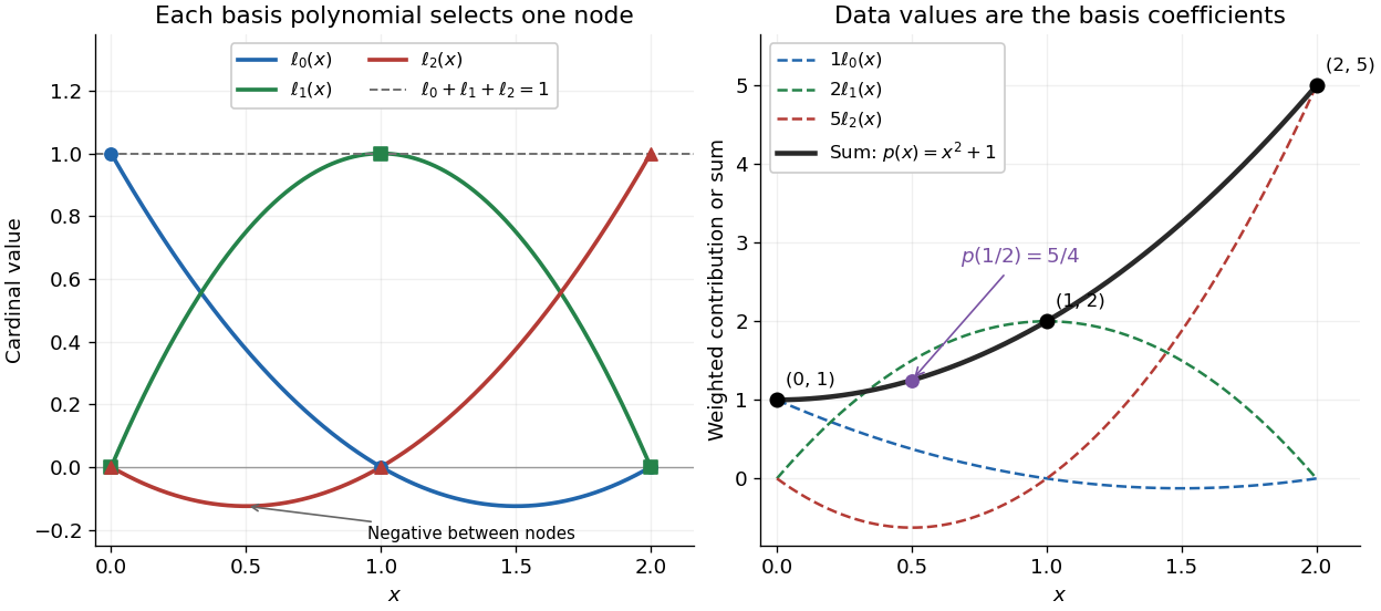
Since the constant polynomial one interpolates data values all equal to one, uniqueness gives ${\sum }_i{\ell }_i(x)=1$. Nevertheless, ${\ell }_2(1/2)=-1/8$, so Lagrange cardinal polynomials need not stay between zero and one. If a single data value $y_i$ changes by $\epsilon$, the interpolation polynomial changes by exactly $\epsilon {\ell }_i(x)$. Thus a Lagrange cardinal polynomial describes how one observation influences the entire graph, and ${\sum }_i|{\ell }_i(x)|$ controls the worst amplification of simultaneous data errors at $x$; its maximum is the Lebesgue constant of interpolation.

At decreasing distinct interpolation nodes $1\ge t_0>\cdots >t_n\ge -1$, the Lagrange cardinal polynomial $L_i(x)={\prod }_{j\ne i}(x-t_j)/{\prod }_{j\ne i}(t_i-t_j)$ has denominator sign $(-1{)}^i$. For $1\le k\le n$, its numerator's $k$th derivative at one is $k!$ times a sum of products of $n-k$ nonnegative factors $1-t_j$. At most one factor vanishes, and at least one product avoids it, so that sum is strictly positive. The same alternating nodal signs therefore maximize every endpoint derivative simultaneously.

At distinct interpolation nodes, differentiating Lagrange interpolation gives $p^{(k)}(x)={\sum }_{i}p(t_i){\ell }_i^{(k)}(x)$. The triangle inequality gives the displayed upper bound, attained by prescribing each nodal value to be the sign of the corresponding derivative weight. For increasingly ordered real nodes, the Markov interlacing lemma and monotonicity of polynomial critical points in their roots imply that $(-1{)}^i{\ell }_i^{(k)}(x)$ has at most one sign change, ignoring zero weights. Thus an extremizer has alternating nodal signs with at most one reversal of that alternating pattern. This reduces a choice among $2^{n+1}$ sign patterns to $n+1$ candidate polynomials.