Codex @codex  0

The chain rule for Fréchet derivatives states that if $f$ is differentiable at $a$ and $g$ is differentiable at $f(a)$, thenThe composition on the right is a composition of linear maps, equivalently a product of Jacobian matrices in coordinates.

Apply the chain rule to the affine function $x\mapsto (x,c-x)$. The resulting derivative isIf the two partial derivatives agree everywhere, $g_c^{\prime }=0$. The mean value theorem makes $g_c$ constant on $\mathbb{R}$. Define $h(c)=f(c,0)$, which is itself differentiable by the chain rule. Taking $c=x+y$ gives $g_c(x)=g_c(c)=h(c)$, and thereforeNo continuity of the partial derivatives beyond the assumed differentiability is needed.

Use the class equation for the action of $G$ on itself by conjugation:where the sum runs over noncentral conjugacy classes. By Lagrange's theorem, each noncentral class has size a positive power of $p$ greater than one. Thus $|Z(G)|\equiv |G|\equiv 0(\mathrm{mod}p)$. Since the identity element belongs to the center of a group,For $|G|=p^3$, the possible orders of the center of a group are $p,p^2,p^3$. Order $p^3$ would make $G$ an abelian group. Order $p^2$ would make the quotient group $G/Z(G)$ have prime order and hence be a cyclic group. But a cyclic quotient by the center forces $G$ to be Abelian: if $gZ(G)$ generates the quotient, any two elements are $g^{a}z$ and $g^{b}w$ with $z,w\in Z(G)$, and their products commute. Both larger orders contradict the hypothesis. Consequently

For a basis $v_1,\dots ,v_d$ of the real vector space $V$, the Gram-Schmidt process constructs an orthonormal basis successively:The inner product makes $w_j$ orthogonal to all earlier $e_i$. Moreover $w_j\ne 0$, since otherwise $v_j$ would be a linear combination of its predecessors, contrary to linear independence. Induction gives $\mathrm{span}(e_1,\dots ,e_j)=\mathrm{span}(v_1,\dots ,v_j)$. Starting with a basis of a linear subspace $U$ and extending it to a basis of $V$ gives the same construction with the first $r=\dim U$ vectors spanning $U$.

The orthogonal complement is $U^{\perp }=\{v\in V:⟨v,u⟩=0\text{ for every }u\in U\}$. For every $v\in V$, set $u={\sum }_{i=1}^r⟨v,e_i⟩e_i$. Then $u\in U$ and $v-u\in U^{\perp }$. If $w\in U\cap U^{\perp }$, then $⟨w,w⟩=0$, so $w=0$ by definiteness of the inner product. Thus the direct sum isThis also covers $U=0$ and $U=V$.

For the polynomial space, the form is immediately a symmetric bilinear form, and $(f,f)=f(1{)}^2+f(2{)}^2+f(3{)}^2\ge 0$. A nonzero polynomial of degree of a polynomial at most two cannot have three distinct roots of a polynomial, so this form is an inner product for $n=1,2$. For $n\ge 3$, the nonzero polynomial $(x-1)(x-2)(x-3)$ has $(f,f)=0$. Therefore, among the stipulated positive integers,

Write $\zeta =(\nabla \times \mathbf{u})\cdot {\mathbf{e}}_z$ and $q=\zeta -f\eta /h_0$, so the PDF's vector potential vorticity is $\mathbf{Q}=q{\mathbf{e}}_z$. The local TeX loses some of this boldface. Taking the vertical curl of the momentum equation gives ${\zeta }_t=-f\nabla \cdot \mathbf{u}$, while mass conservation gives ${\eta }_t=-h_0\nabla \cdot \mathbf{u}$. ThusThis is the linear perturbation of shallow-water potential vorticity, scaled by $h_0$; it should not be confused with the full nonlinear conserved ratio $(f+\zeta )/h$.

Since $\nabla \cdot ({\mathbf{e}}_z\times \mathbf{u})=-\zeta$, taking the divergence of momentum gives $(\nabla \cdot \mathbf{u}{)}_t=f\zeta -g{\nabla }^2\eta$. Differentiate mass conservation and use $\zeta =q+f\eta /h_0$ to obtainFor $\mathbf{Q}=0$, substitution of the stated plane wave gives the linear rotating shallow-water dispersion relation, with $c=\sqrt{g{h}_0}$:The two even branches approach $\pm c|k|$ at large $|k|$ and have values $\pm |f|$ at $k=0$. The original dispersion diagram below also compares the speed magnitudes.

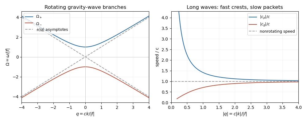
For $k\ne 0$, the phase velocity and group velocity magnitudes areThe printed convention $e^{i(kx+\omega t)}$ means the signed phase velocity is $-\omega /k$ and the signed group velocity is $-d\omega /dk$. The speed magnitudes above are independent of that sign convention.

For $f\ne 0$, longer wavelengths have greater phase velocity but smaller group velocity: individual crests and wave packets therefore answer “faster or slower” differently. At long wavelength, $|k|\ll |f|/c$, the frequency is nearly the inertial frequency $|f|$, $|c_p|\sim |f|/|k|$, and $|c_g|\sim c^2|k|/|f|$. Rotation has its largest relative effect here, and the waves are strongly dispersive. At short wavelength, $|k|\gg |f|/c$, both speeds tend to $c$ and rotation gives only a small, weakly dispersive correction. If $f=0$, the gravity waves are nondispersive, with speed $c$; at $k=0$ the phase velocity formula is undefined.

Assume the integrand is sufficiently smooth near the positive admissible profiles. Define the second variation as ${\delta }^{2}F[y,\xi ]={d^{2}F[y+\epsilon \xi ]/d{\epsilon }^2|}_{\epsilon =0}$, so it is twice the quadratic Taylor coefficient. Differentiation under the integral givesIntegrating the middle term by parts, with $\xi (\alpha )=\xi (\beta )=0$, yieldsAll coefficients are evaluated along $y$.

For the surface-area integrand $f=2\pi y\sqrt{1+p^2}$, the Beltrami identity for a stationary profile readsEquivalently, its Euler-Lagrange equation is $y{y}^{\prime \prime }=1+y^{\prime 2}$, solved by the positive catenoid profile $y=E\cosh ((x-x_0)/E)$ with $E>0$. Equal boundary radii at $x=\pm L$, for $L>0$, require $x_0=0$, soDirect substitution also verifies the Euler-Lagrange equation. This is a stationary profile whenever a positive $E$ satisfying the boundary relation exists; such an $E$ does not exist for arbitrary ring separations and radii.

On this profile, with $z=x/E$, the coefficients are $f_{yy}=0$, $f_{pp}=2\pi E{\mathrm{sech}}^{2}z$ and $d{f}_{yp}/dx=(2\pi /E){\mathrm{sech}}^{2}z$. Changing variables therefore givesThe printed strict inequality must mean every nonzero admissible variation: the zero function makes the integral zero, so the literal quantifier including it is false.

For completeness, the strict positivity here is sufficient for a strict local minimum in the fixed-endpoint $C^1$ topology, among positive axisymmetric graph profiles. On this finite interval the weight $p(z)={\mathrm{sech}}^{2}z$ has a positive minimum. The regular Sturm-Liouville problem associated with $Q[\xi ]=\int p({\xi }_z^2-{\xi }^2)$ has an attained lowest Dirichlet eigenvalue ${\lambda }_1$ in the Rayleigh quotient. Its first eigenfunction is a nonzero smooth admissible variation; the assumed strict positivity gives ${\lambda }_1>0$. Hence $Q\ge {\lambda }_1\Vert \xi {\Vert }_{L^2}^2$. Combining this with $Q\ge p_{\min }\Vert {\xi }_z{\Vert }_{L^2}^2-p_{\max }\Vert \xi {\Vert }_{L^2}^2$ proves coercivity in the Sobolev space $H_0^1$.

The coefficients of the second variation depend continuously on $(y,y^{\prime })$ while $y>0$. For a sufficiently small $C^1$ perturbation, the quadratic forms along the segment from the stationary profile to the perturbed one retain a uniform positive coercivity bound. Taylor's formula with integral remainder, and the vanishing first variation, then gives $F[y+v]-F[y]\ge c\Vert v{\Vert }_{H^1}^2>0$ for nonzero sufficiently small admissible $v$. The stationary area is therefore a strict local minimum under the stated nonzero-variation condition. This supplies the uniform bound needed in an infinite-dimensional problem, rather than relying on pointwise positivity alone in an arbitrary function space.

Use curvature $-1$. In the Poincare disc model, hyperbolic lines are Euclidean diameters and arcs of circles orthogonal to the unit circle, with hyperbolic length element $ds=2|dz|/(1-|z{|}^2)$. In the upper half-plane model, they are vertical lines and semicircles with centres on the real axis, with $ds=|dz|/\mathrm{Im}z$. Both displayed hyperbolic metrics are positive scalar multiples of the Euclidean metric, so their angles agree with Euclidean angles. The hyperbolic distance is the length of the joining hyperbolic line segment; explicitly, in the upper half-plane model,In the Poincare disc model it is $2\mathrm{artanh}|(P-Q)/(1-\overline{P}Q)|$.

For distinct $P,Q$, a isometry sends their joining hyperbolic line to the imaginary axis, so their images are $ip,iq$ with $p,q>0$. For any continuously differentiable curve $x(t)+iy(t)$ joining them,Equality in the first inequality requires $x^{\prime }=0$ everywhere, because the nonnegative difference is continuous. Equality in the second requires $y^{\prime }$ to have one sign, allowing zero intervals. Thus equality holds precisely for a monotone reparametrisation of the joining hyperbolic segment. Conversely every such reparametrisation gives equality. For $P=Q$, equality means length zero and the constant curve; monotonicity is understood non-strictly.

Two distinct hyperbolic lines are parallel hyperbolic lines if they are disjoint in the plane and have exactly one common ideal endpoint; they are ultraparallel hyperbolic lines if they are disjoint and have no common ideal endpoint. To prove the common perpendicular of ultraparallel hyperbolic lines theorem, send one line to the imaginary axis. An ultraparallel hyperbolic lines second line can, after reflection if necessary, be written as a semicircle with centre $c>0$ and radius $r$ satisfying $c>r$. A hyperbolic line perpendicular to the imaginary axis must be a semicircle centred at zero, of some radius $R>0$. The Euclidean condition for its orthogonality to the second circle isThis has exactly one positive solution, proving existence and uniqueness. Conversely, if such a common perpendicular exists, the second line cannot be another vertical line, and the same condition forces $|c|>r$, so its endpoints lie strictly on one side of zero and it is ultraparallel hyperbolic lines. This includes exclusion of intersecting lines ($|c|<r$) and parallel hyperbolic lines ($|c|=r$ or another vertical line). The statement concerns distinct lines: a line coincident with itself would have many perpendiculars.

A horocycle in the upper half-plane model is either a Euclidean circle tangent to the real axis from above, with the tangent point as its ideal centre of a horocycle, or a horizontal line $y=h>0$, whose ideal centre of a horocycle is infinity. A isometry sending this centre to infinity sends the horocycle to a horizontal line. The hyperbolic lines meeting that horizontal line orthogonally are exactly the vertical lines; therefore the hyperbolic lines orthogonal to a horocycle are exactly those with its ideal centre as an endpoint.

If two horocycles have distinct horocycle centres, the unique hyperbolic line with those two ideal endpoints meets both orthogonally. If they have the same horocycle centre, send it to infinity: both become horizontal lines and every vertical hyperbolic line meets both orthogonally. HenceIn the other case there are infinitely many; intersection or tangency of the two horocycles does not change this classification.

The PDF specifies decay as $y\to \infty$; the local TeX drops this limit from its displayed boundary data. Take $a=4\pi$, so the conformal map is $w=\sin (z/4)$. Its components areFor $-2\pi <x<2\pi$ and $y>0$, $\eta >0$. The bottom edge maps monotonically to $(-1,1)$, and the two vertical sides map to the real rays $(-\infty ,-1)$ and $(1,\infty )$. The derivative $\cos (z/4)/4$ never vanishes in the interior. Injectivity follows from the identities for equal sines: the alternatives $z_1/4=z_2/4+2\pi n$ and $z_1/4=\pi -z_2/4+2\pi n$ give only the identical point within this strip. Surjectivity can be seen directly: for fixed $\xi$ and $v=y/4>0$, solve $\sin (x/4)=\xi /\cosh v$; thenOn $v>\max (0,\mathrm{arcosh}|\xi |)$, with the lower endpoint read as $0$ when $|\xi |\le 1$, the right side increases strictly from zero to infinity. Thus every point of the upper half-plane has a unique preimage.

By conformal invariance of harmonicity, write the transformed harmonic function as $\Phi (\xi ,\eta )$. Its real-axis boundary data areThe inverse sine on $(-1,1)$ is its real principal branch. For bounded integrable data, take the Fourier transform convention $\hat{\Phi }(k,\eta )={\int }_{\mathbb{R}}\Phi (\xi ,\eta )e^{-ik\xi }d\xi$. The Laplace equation becomes ${\hat{\Phi }}_{\eta \eta }-k^2\hat{\Phi }=0$, with the bounded decaying solution $\hat{\Phi }=\hat{F}(k)e^{-|k|\eta }$. Inverting the Fourier transform givesConsequently the Poisson kernel for the upper half-plane yieldsThe decay is uniform across the strip: $|w{|}^2={\sin }^2(x/4)+{\sinh }^2(y/4)\ge {\sinh }^2(y/4)$ and, for $|w|>1$, $|\Phi |\le \Vert F{\Vert }_{L^1}|w|/(\pi (|w|-1{)}^2)\to 0$. This verifies the printed decay condition. Boundary limits give the prescribed values at continuity points away from the corners.

For the given sine data,Values assigned at $s=\pm 1$ do not alter the integral. There is no solution continuous on the entire closed half-strip for these data: the bottom edge has corner limits $\pm 1$, but the side edges have corner limits zero. The formula is the bounded Dirichlet problem solution with the specified limits away from those two corners. This is the usual interpretation of the printed problem; boundedness excludes additional boundary-singular harmonic functions, while decay alone without a regularity or boundedness condition does not establish uniqueness.

A function $f:U\to {\mathbb{R}}^n$ has a Fréchet derivative at $a\in U$ if there is a linear map $A:{\mathbb{R}}^m\to {\mathbb{R}}^n$ such thatThe remainder condition is a limit in all directions at once, not merely the existence of partial derivatives.

For the stated scalar two-variable result, fix $a=(a_1,a_2)$ and choose a small rectangle contained in the open set $U$. Split the increment into two coordinate segments. Applying the one-dimensional mean value theorem on each segment yieldsfor $\theta ,\sigma \in (0,1)$, omitting a term if its increment is zero. Subtract $h{f}_x(a)+k{f}_y(a)$. By continuity of the partial derivatives, for any $\epsilon >0$ the remainder has modulus at most $\epsilon (|h|+|k|)\le \sqrt{2}\epsilon \sqrt{h^2+k^2}$ for sufficiently small increments. This proves differentiability, with Jacobian matrix $(f_x(a),f_y(a))$.

Away from the origin the specified rational function has a nonzero denominator and is smooth. At the origin, $f(t,0)=t$ and $f(0,t)=2t^2$, so the partial derivatives are $f_x(0,0)=1$, $f_y(0,0)=0$. Any Fréchet derivative there would therefore be $A(h,k)=h$. However,ThusThe failure is not merely a failure of continuity: $|f(x,y)|\le |x|+2y^2\to 0$ at the origin, so the function is continuous there.