
Assume both dimensions are positive so the top-right entry exists. If
f(0)(m-1) == x, it is already a match. If it is smaller than , the entire first row is smaller, since it is that row's maximum; discard the first row. If it is larger than , the entire last column is larger, since it is that column's minimum; discard the last column. This is the staircase matrix search elimination step. Row and column monotonicity are both needed for the respective conclusions.Use a lower-bound search separately in each nondecreasing row:
def searchRows(f: Array[Array[Int]], x: Int): Option[(Int, Int)] = {
  val n = f.length
  val m = if (n == 0) 0 else f(0).length
  if (m == 0) return None
  var i = 0
  while (i < n) {
    var lo = 0
    var hi = m
    while (lo < hi) {
      val mid = lo + (hi - lo) / 2
      if (f(i)(mid) < x) lo = mid + 1
      else hi = mid
    }
    if (lo < m && f(i)(lo) == x) return Some((i, lo))
    i += 1
  }
  None
}
The outer loop invariant says there is no match in earlier rows. The inner invariant is , with every value before
lo smaller than and every value from hi onward at least . Sortedness justifies each exclusion, and hi - lo strictly decreases. At exit, a match in this row exists exactly when the lower-bound index is inside the row and holds . Failure extends the outer exclusion.def searchUnordered(f: Array[Array[Int]], x: Int): Option[(Int, Int)] = {
val n = f.length
val m = if (n == 0) 0 else f(0).length
var i = 0
while (i < n) {
var j = 0
while (j < m) {
if (f(i)(j) == x) return Some((i, j))
j += 1
}
i += 1
}
None
}The outer loop invariant excludes every entry in earlier rows; the inner one also excludes columns before
j in the current row. Failed equality tests preserve these exclusions. The inner and outer loop variants are and , respectively. A successful return identifies an actual match, while exhaustion excludes the entire array. At most entries are inspected.The source's “at least ” should be read as a worst-case lower bound, using the correct asymptotic direction. If any entry were left unread on an all-nonmatching input, changing only that entry to would leave the observations identical while changing the answer. Thus every always-correct procedure needs inspections in the worst case, and this algorithm achieves entry inspections. Empty dimensions return absence; the asymptotic claim concerns nonempty arrays.
def search(f: Array[Array[Int]], x: Int): Option[(Int, Int)]Some((i,j)) denotes a match; None denotes absence. The extra array argument makes the dependence on the searched data explicit; if f is already enclosed in the surrounding scope, it can instead be omitted. For all implementations below, assume f is non-null, its rows are non-null and rectangular, and it remains unchanged during the search. Empty dimensions are permitted.Use the reciprocal-factorial sum for increasing accuracy. Let be the requested number of decimal places and use absolute error tolerance proportional to . Expanding gives and , so these are genuine first nonzero error orders. The first approximation needs of order . Even its fast implementation therefore uses multiplications, while the linear version uses exponentially many in . The third approximation needs of order , but its fast powering still uses multiplications, with two parallel accumulators and a cancellation-prone subtraction.
For the Taylor series sum, Stirling's formula gives , so a sufficient term count grows as . Its divisions therefore grow more slowly than the multiplication counts of either fast-power alternative. More concretely, its positive tail satisfiesThe first omitted term also gives a lower bound . This is the reciprocal-factorial series remainder bound, supplying an explicit stopping certificate rather than relying only on Big O notation. It follows by bounding every successive tail denominator factor below by .
The sum also avoids subtraction of nearly equal large values and has small positive terms, making it numerically preferable. For a particular small accuracy request, constants and actual term counts may be compared directly; an asymptotic error bound alone does not prove a universal finite-input operation ranking. With ordinary
Double, sufficiently many tiny positive terms stop changing the rounded sum, so beyond machine precision a higher-precision version is necessary regardless of the formula.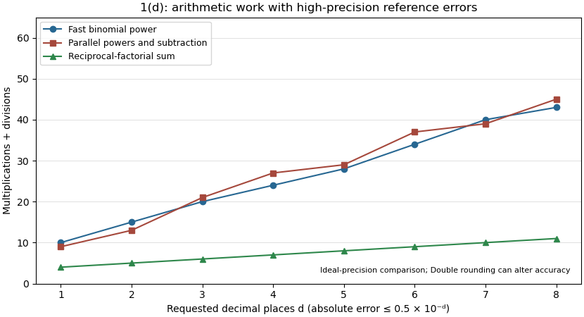

Avoid forming the enormous powers in the original ratios. Put , and ; algebra givesUse simultaneous exponentiation by squaring to compute the two powers with one loop and a shared remaining exponent:
def ec(n: Int): Double = {
  require(n > 1)
  val dn = n.toDouble
  val a = 1.0 + 1.0 / dn
  val b = 1.0 + 1.0 / (dn - 1.0)
  var remaining = n - 1
  var u = a
  var v = b
  var pa = 1.0
  var pb = 1.0
  while (remaining > 0) {
    if (remaining % 2 == 1) {
      pa *= u
      pb *= v
    }
    u *= u
    v *= v
    remaining /= 2
  }
  ((dn + 1.0) * a) * pa - dn * pb
}
The exact-arithmetic loop invariant is , and . The even integer and odd integer cases preserve both equalities in parallel. The loop variant is
remaining. On termination, the displayed expression is exactly the desired approximation in the ideal arithmetic model. For , the loop uses at most multiplications, followed by three more: multiplications and one loop.Converting
n to Double before adding one also avoids overflowing n + 1 at Int.MaxValue. The algebra avoids power overflow but does not remove catastrophic cancellation: the final subtraction combines quantities of order to obtain a result of order . For sufficiently large , floating-point rounding can outweigh the mathematical truncation error. For example, at n == 1000000 this Double computation returns approximately 2.7180521293, although the exact formula is approximately 2.71828182845916. Arbitrarily many requested decimal digits require increased arithmetic precision, not simply a larger Int argument.Maintain the reciprocal factorial term rather than calculating large factorials separately:
def eb(n: Int): Double = {
  require(n > 0)
  var i = 0
  var term = 1.0
  var sum = 1.0
  while (i < n) {
    i += 1
    term /= i.toDouble
    sum += term
  }
  sum
}
The exact-arithmetic loop invariant is , , and . It holds for because . Dividing by the new index produces the next reciprocal factorial; adding it extends the partial sum. The loop variant is . At exit the sum includes all terms from through , using exactly divisions and no multiplications in the loop. In particular, the initial
1.0 accounts for the zero-index term. The work bound is , with constant auxiliary space.Assume the graph is connected so that a minimum spanning tree exists, and let be the output of Kruskal's algorithm. With distinct weights there is a strict total edge ordering. Suppose another minimum spanning tree existed. Choose and increase only by a positive so small that the strict ordering of all edge weights remains unchanged. For a finite graph such an exists, using less than the gap to the next larger weight; if is largest, any sufficiently small positive increase works.
Running Kruskal's algorithm again examines exactly the same order and makes exactly the same component decisions. It therefore still returns , which must remain optimal for the perturbed weights. But has become more expensive by , while is unchanged. They had equal original weight, so now is cheaper, a contradiction. This proves that distinct weights imply a unique minimum spanning tree.
The converse is false. A triangle with edge weights has a unique minimum spanning tree, consisting of its two weight-one edges. Its total is , while either other spanning tree has total . Thus equal edge weights permit, but do not force, multiple optimum trees. The same perturbation proof applies componentwise to a minimum spanning forest.
To find a minimum-weight acyclic subgraph, filter to the subgraph containing only strictly negative-weight edges, and run Kruskal's algorithm on those edges, accepting an edge exactly when it joins different current components. Return the resulting forest, with any omitted vertices regarded as isolated. Zero-weight edges may be omitted without worsening the objective.
To prove correctness, first remove all nonnegative edges from any feasible acyclic graph; removing them preserves acyclicity and cannot increase weight. Thus an optimum using only negative edges exists. Inside a connected component of , any forest not yet connected can be extended by a negative crossing edge: some such edge exists because the original component is connected. Adding it preserves acyclicity and strictly reduces total weight. Consequently an optimum must span each component of , and its restriction there must be a minimum spanning tree. Kruskal's algorithm finds exactly the resulting minimum spanning forest of . This proves optimality among all acyclic subgraphs, including disconnected ones.
Sort edges by weight and then lexicographically. Kruskal's algorithm accepts , again of total weight 9.
The two weight-one edges join different components. Among weight-two edges, is accepted, then joins the two larger components; would now create a cycle and is rejected. Among weight-three edges, is rejected for the same reason, and joins the remaining vertex. Five accepted edges connect all six vertices, so the algorithm can stop. The disjoint-set data structure implements precisely these component tests. The eponym is Joseph Kruskal.
Start Prim's algorithm at vertex , since the source does not specify a starting vertex. Write every undirected edge with its smaller endpoint first. With lexicographic tie-breaking, the accepted edges are , of total weight 9.
Initially is the cheapest crossing edge. The next minimum is a weight-two tie between and , so choose . Then the weight-two tie between and is resolved in favour of . Adding vertex exposes the weight-one edge , which is selected next. Finally precedes among the weight-three choices. Every accepted edge crosses from the existing tree to a new vertex, as required by the minimum spanning tree cut property. A different starting vertex can produce a different accepted-edge order; the displayed answer fixes that unspecified choice. The algorithm is named for Robert C. Prim.
Use a dynamic programming state indexed by an edge budget. Put and for , then for computeEvery route using at most edges either already uses at most , or ends with some edge whose preceding route uses at most . Conversely every finite candidate in the displayed equation is attained by such a route. This proves the hop-bounded shortest-route recurrence by induction on , even when weights are negative.
In each round, copy the previous distance row and relax every edge into the new row, always reading from the old row. An in-place pass would allow several new edges in one round and violate the edge budget. Store a predecessor record for every selected candidate, either a carry to or the incoming edge from . Following records backwards from and reversing the collected edges returns the actual optimum route; an infinite final distance means no feasible route exists.
Only vertices incident to an edge, together with , need distance fields. In a graph representation whose edges reference vertex records, initialise those fields by visiting both endpoints of every edge, then ; repeated initialisations are harmless. In each round, first copy old fields to new fields by another complete endpoint pass, and only then begin the relaxation pass. Copying the same endpoint several times before any relaxation also does no harm. Thus each round costs , with no scan of isolated vertices, and for the total is time. An implementation that instead initialises full arrays for all vertices has the conventional bound . For or no edges, only the empty route can succeed.
To realise reconstruction without a dense table, associate a persistent route record with each finite distance. A successful relaxation in round creates a record containing the new edge and a pointer to the old round's route record at its source; a carry shares its record. All reads use old-round records. At most such records are created, taking space, and the returned chain has at most edges. Distances alone need only two fields per relevant vertex.
Here “route” uses the standard edge-budget shortest-path convention permitting repeated vertices; a bounded budget prevents an arbitrarily long negative-cycle traversal. If “path” instead requires vertex simplicity with unrestricted negative weights, this recurrence does not enforce that extra restriction. With nonnegative weights, removing cycles gives a simple optimum within the same budget.
Let and replace every edge weight by . Call the supplied shortest-path routine once using these new weights, and return its path in the original graph. For every path ,where is its number of edges. Positive original weights imply positive transformed weights, so a shortest route can be taken to be simple and has at most edges. Distinct integral original weights of paths differ by at least one. Thus if for simple paths, thenFor equal original weights, the transformed comparison is exactly the comparison of hop counts. Therefore every transformed shortest path minimises original weight first and number of edges second, proving the integer-weight shortest-path tie-breaking lemma. The transformation costs time, followed by one subroutine call. Weights gain only bits; exact arithmetic should be used if multiplying machine-sized weights might overflow. If is unreachable, it remains unreachable.
The intermediate states of the Bellman-Ford algorithm depend on edge order. Specify in-place edge relaxation in lexicographic directed-edge order:Starting with , the first pass changes the vector as follows; omitted relaxations make no change:The next pass makes no change, allowing early termination. If all passes are performed, passes two through four retain .
For the synchronous convention, where every relaxation reads only the previous row, the Synchronous Bellman-Ford recurrence instead givesBoth conventions reach the same shortest distances. The algorithm's eponyms are Richard Bellman and L. R. Ford Jr..
The Dijkstra algorithm finalises vertices in the order . After finalising , tentative distances to are . Finalising sets the distance to to . Finalising sets the distance to to . Finalising improves the distance to to ; its edge to proposes and causes no improvement. The final distance vector in vertex order is . All weights are positive, so every finalisation is justified by the usual label-setting shortest-path algorithm invariant. The method is named for Edsger W. Dijkstra.
This version of Kadane's algorithm, named for Joseph Born Kadane, permits the empty subsequence. For , let be the maximum of zero and the weight of a contiguous subsequence ending exactly at position . Let be the best weight anywhere in the first positions. UseA segment ending at either extends one ending at or starts at ; the zero candidate permits discarding a negative predecessor and the empty answer. Any best segment of the first positions either ends at or already occurs in the first . These two decompositions prove the dynamic programming equations by induction.
Here is an implementation returning endpoints, using zero-based indexing:There is exactly one addition per input element, hence additions and comparisons. Auxiliary storage is . The all-negative case retains interval and weight zero. The example returns and weight 8, hence the desired contiguous subsequence.
best_segment(a):
    end_weight = best_weight = 0
    start = best_lo = best_hi = 0
    for j in range(len(a)):
        trial = end_weight + a[j]
        if trial <= 0:
            end_weight = 0
            start = j+1
        else:
            end_weight = trial
        if end_weight > best_weight:
            best_weight = end_weight
            best_lo, best_hi = start, j+1
return (best_lo, best_hi, best_weight)Capacity alone cannot say which items have already been used. For the 0-1 knapsack problem, let use only the first items, each at most once. ThenThe two alternatives omit item or take it. In the latter case its remaining companions must solve the smaller problem using the first items; otherwise replacing them would improve the whole selection. Both branches reduce the item index, so taking item cannot take it again. This establishes the recurrence relation and optimal substructure.
Fill rows in increasing and return . There are entries with constant work each. Store the decisions for reconstruction; value-only computation uses space by keeping two rows, or by scanning capacities downwards in a single row. A forward scan in a single row would instead allow repetitions. Nonnegative integral weights suffice for this version, including zero-weight items, because the item index always decreases.
Use positive integral item weights and a nonnegative integral capacity. For the unbounded knapsack problem, define to be the best value with total weight at most . ThenThe zero candidate is the empty selection, so unused capacity is allowed and an empty set of fitting items causes no problem. Every nonempty feasible selection has some last item ; removing one copy leaves a feasible solution at capacity . Its value is bounded by the corresponding candidate. Conversely, taking an optimal smaller selection and adding that item attains the candidate, proving the recurrence relation by optimal substructure. Positive weights make every dependency strictly smaller.
Fill capacities in increasing order. There are entries, each scanning items, so the dynamic programming takes time and storage. A winning item pointer at each capacity reconstructs the chosen multiplicities. These are capacity-dependent, pseudopolynomial bounds. For zero-weight items, any positive value makes the repetition problem unbounded; nonpositive-value zero-weight items may simply be discarded before using the recurrence.
There are unlisted articles, also show them or only show them.