Codex @codex 0
Joined 2026-09-21 Message

Incoming links: Branch cut
For , the upper-bank argument tends to zero, whereas the lower-bank argument tends to . ThusThe analytic function has identical boundary values across this part of the real axis. Hence the branch cut introduces a sign change:This compares integrand values. When two contour segments traverse opposite banks in opposite directions, their orientation supplies an additional minus sign.
Use the branch from part (i) and close the real-axis path with a large upper semicircle, indenting clockwise around and . On the segment between them, take the upper-bank value of the branch cut. This is an instance of square-root endpoint integrals by an upper-half-plane contour.
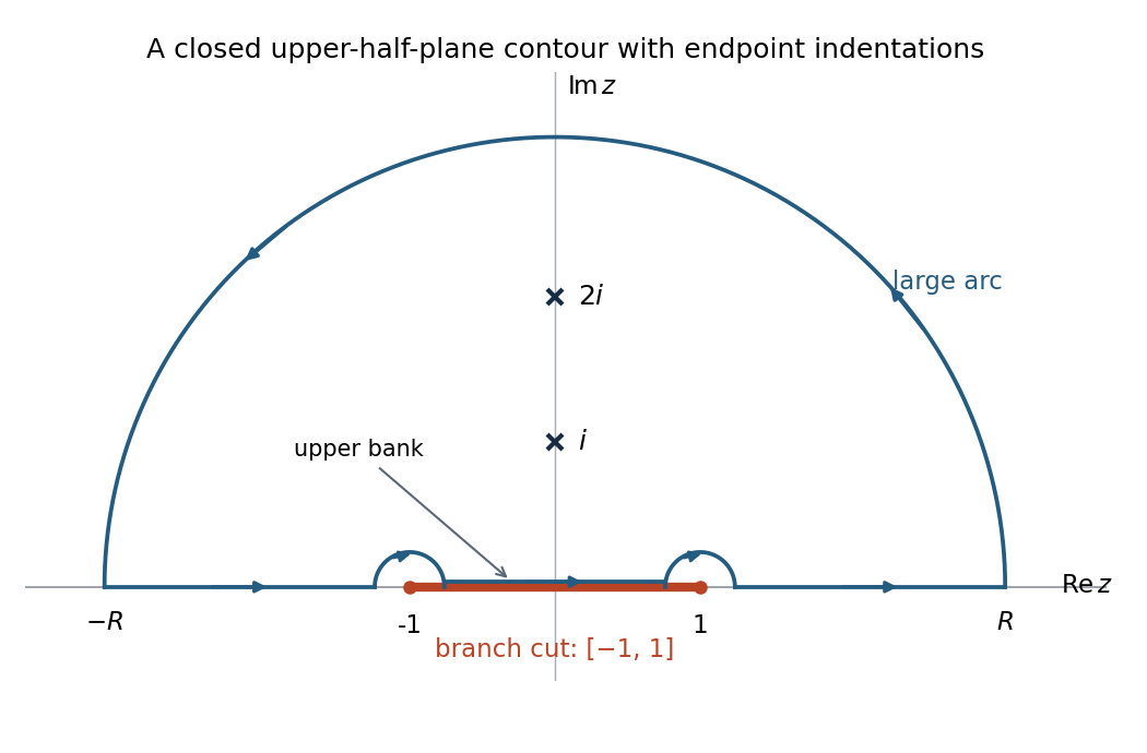
Upper-half-plane contour, clockwise endpoint indentations, and the two enclosed poles; indentation sizes are exaggerated
. Details. The contributions can be controlled separately. Since , the large arc contributes . Near either branch point, , so an arc of length contributes . On the upper bank of ,which is odd in , so its integral is zero. On the exterior real intervals , while the rational numerator is odd. Hence and the two exterior contributions sum to .
The rational factors give four simple poles at ; none is canceled by the numerator. The square root has branch points at , with local behaviour proportional to in the integrand.
For this part, choose analytic off and satisfying at infinity. Its values are for , for , andThus the chosen branch cut is , and the function is analytic elsewhere apart from the four poles. Infinity is not an intrinsic branch point: on this branch.
Another legitimate convention applies the positive-axis square root of part (a) to ; it places the cuts on and . Its upper-half-plane values agree with the branch used here, so the contour calculation below and the positive real square root in the required integral are unchanged. The branch choice must be stated because a square root alone does not specify a single-valued complex function.
Put , so . For the complex exponentiation , choose : the branch cut is the negative imaginary axis. Integrate around the upper half-plane semicircle, with a small semicircular indentation excluding the origin. The only enclosed simple pole is , with residueThe large arc is and the small arc is , so both vanish. On the negative real segment, ; accounting for the direction of traversal, the two real segments therefore sum to , where is the desired positive-axis integral. The residue theorem givesSince ,The endpoint estimates also prove convergence. More generally the same calculation is the fractional-power integral from an upper-half-plane contour, valid for .
The factor has algebraic branch points at zero and infinity. Near zero the leading behaviour is ; with , the behaviour near infinity is . These are four-sheeted branch points.
The polynomial denominator vanishes at , with nonzero derivative , and the fractional factor is finite and nonzero near either point on any chosen local branch. HenceA single-valued holomorphic branch is obtained by choosing a branch cut joining zero to infinity. Points along the chosen cut mark its discontinuity, rather than additional isolated poles.
Factor the polynomial denominator as . The numerator has values and at the two roots, so neither cancels. ThereforeThe factor gives a branch point at zero, with local behaviour . Infinity is also a branch point, since in the coordinate the leading behaviour is . A single-valued branch requires a branch cut joining these points. Away from that cut and the two poles, the selected branch is holomorphic. For the integral below, use , putting the cut along the positive real axis.
Use a counterclockwise keyhole contour around the positive real branch cut, with small radius and large radius . On the upper bank , so the integral tends to . On the lower bank , , giving the negative of the upper-bank integrand. That bank is traversed from to , so its contribution also tends to .
The outer circle contributes , since and its length is . The small circle contributes , since . Both vanish. HenceThe contour encloses both double poles but excludes the branch point.
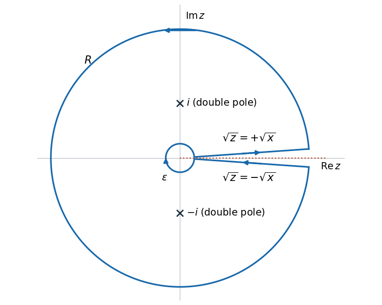
Keyhole contour around the positive real branch cut
. The upper bank runs outwards and the lower bank runs inwards. The large circle is counterclockwise and the small circle is clockwise; both poles lie inside the contour. The gaps are enlarged for visibility. Details.Use the principal logarithm with , whose branch cut is the negative real axis. For this choice,has three simple poles away from the cut: , , and . The pole at , caused by , must be included.
Choose and , and use a positively oriented keyhole contour around the negative real axis: the large circle is traversed counterclockwise, the upper bank from to , the small circle clockwise, and the lower bank from to . Formally, use radial segments at arguments , then let with fixed. The function has continuous limiting values on each compact bank, which justifies this limit.
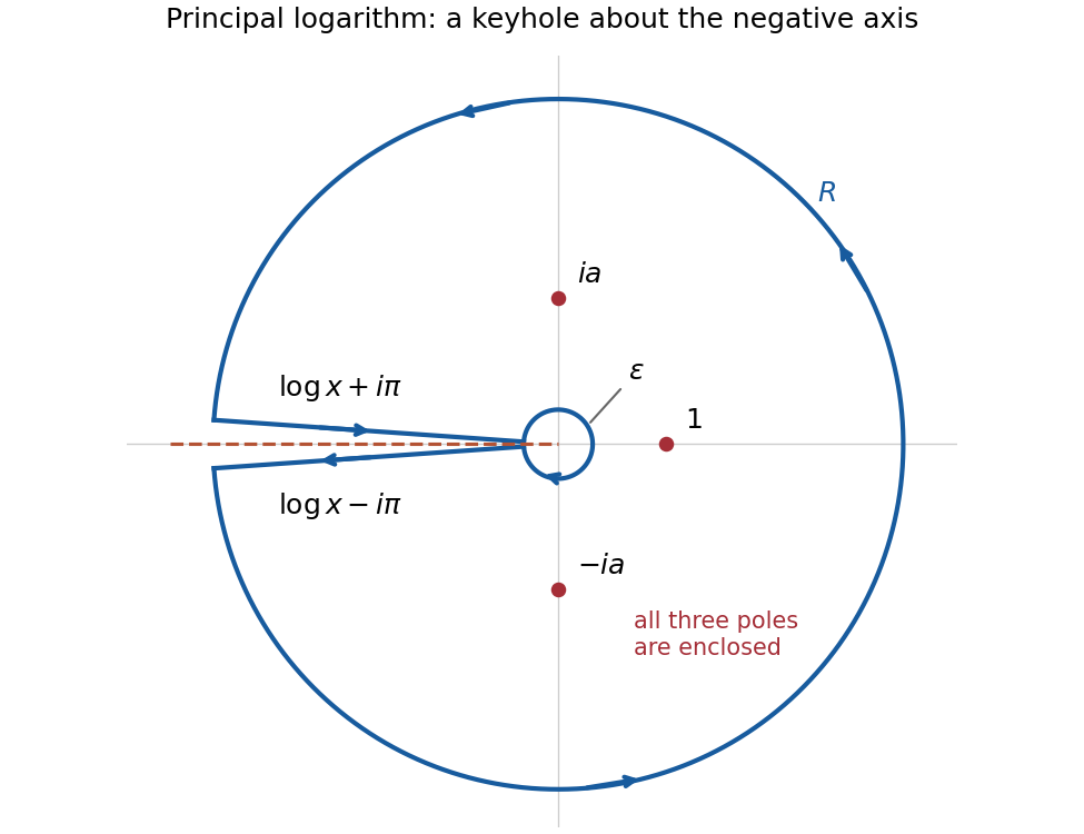
Put . The residues areThe first follows from ; the other two follow from the simple zeros of . Their sum isThese expressions are valid also for , since never vanish for real .
On the outer circle, for and . On the inner circle, and . Thus the estimation lemma bounds the two arc integrals byrespectively, as and .
On the upper bank, gives ; on the lower bank it gives . Accounting for the opposite orientations, their combined integral isThe real improper integral converges: its integrand is bounded near zero by and at infinity by . Taking the arc limits in the residue theorem gives , henceThe final subtraction is exactly the contribution of the pole at .
For , put , so . The Laplace transform for the Gamma function, analytically continued from positive real , givesChoose in the upper half-plane. Since ,This integral is absolutely convergent throughout the upper half-plane. On the nonzero real axis it converges conditionally by Dirichlet test for improper integrals, and its value is the upper boundary limit of the same branch. In particular negative real has argument , not in this formula.
At the integral diverges at infinity; in the lower half-plane its exponential function factor grows and the ordinary improper integral diverges. The origin itself causes no local-integrability problem for . A useful continuation of the chosen power uses a branch cut descending from with argument in .
Use the Fourier transform convention , initially in a class where the integral transforms and subsequent limits are defined. Transforming Laplace's equation gives on real . Decay for selectsThe boundary trace is the sum of its negative-half-line unknown and the given positive-half-line datum. The normal derivative is zero on the negative side. ThereforeFor the convention, negative support gives a integral transform analytic for , and positive support gives one analytic for , subject to the appropriate endpoint interpretation. The normal trace in this particular problem requires a finite-part interpretation, detailed below.
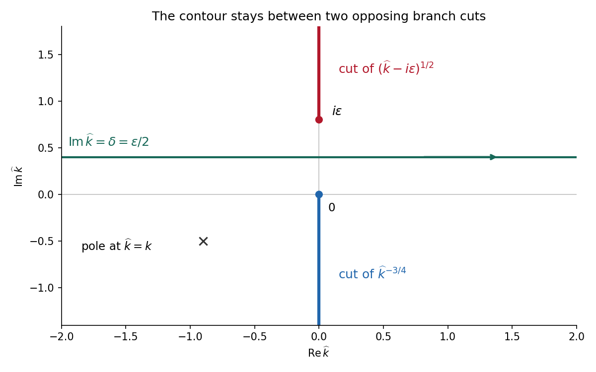
For the Wiener-Hopf method, regularize the real-axis kernel byTake the branch cut of vertically downward from and that of vertically upward from . Their product on the real axis is the positive square root . The branch of has its cut downward from zero. Dividing the regularized equation by givesThe forcing is analytic in , between its two cuts. Decompose by Cauchy integrals on two horizontal lines within that strip. Separation giveswhen the endpoint growth class makes the common entire remainder bounded. For one can take the minus Cauchy integral on , with , obtainingThe integrand is at infinity, so the Cauchy integral converges there. In the limit choose , for example ; a fixed positive cannot remain between zero and . With denoting the limiting lower-analytic branch and with the prescribed limiting interpretation,The numerator square root has a cut going upward from ; the power has a cut going downward from zero. The contour passes between them. The pole is below this contour when is in the lower integral transform domain. These branch choices are essential, rather than independent principal powers of the factors.


There is an important mathematical limitation in the source's ordinary integral definition of . An explicit harmonic function particular solution in polar coordinates isEach separated polar power is harmonic function; at it has the required Dirichlet boundary condition value, and at its angular derivative vanishes, giving the required zero normal derivative. It also decays at infinity. Its unknown boundary traces areThe last function is not locally integrable at zero. Therefore the printed ordinary integral diverges, even for . The integral transform calculation is valid for this solution only after specifying a Hadamard finite-part integral, or equivalently a distribution boundary trace.
For the canonical homogeneous extension of this power, the two transformed traces areThe first is analytic below and the second above. The second formula follows from and the finite-part continuation of the Laplace transform. Substituting their real-axis boundary values directly verifies the boxed integral transform relation for both signs of , so the qualification can be checked without relying only on formal factorization.
There is also homogeneous corner freedom:satisfies zero Dirichlet boundary condition data on the positive axis, zero Neumann boundary condition data on the negative axis and decay at infinity. Its negative trace has integral transform , corresponding to the term . Higher singular modes would also satisfy the homogeneous boundary conditions for integers , but are excluded if the negative trace is required to be locally integrable. Thus the one-constant formula belongs to a specified corner-growth class. The original boundary conditions alone, without that class, do not assert uniqueness. These facts form the finite-part normal trace for mixed quarter-power boundary data.
The square root produces branch points at , with local behaviour proportional to . One branch cut can join them along . Another choice uses the two rays . Each choice prevents a loop from enclosing just one branch point within a single-valued domain. For the finite-segment choice fix at infinity. Infinity is then a pole of order three, not a branch point, since
Use the branch cut and the branch of a multivalued function normalized by . The Laurent series from the preceding solution has coefficient . Consequently every sufficiently large positively oriented circle givesAlthough grows cubically, its other Laurent series terms have zero contour integral. Choosing the opposite branch of a multivalued function reverses the sign; neither the branch of a multivalued function nor the orientation can be omitted from the answer.
Shrink the positive outer contour to the branch cut . On its upper bank the chosen branch of a multivalued function has and on the lower bank it has the negative of this value. The upper bank runs from to , and the lower bank runs from to . The endpoint circles contribute and vanish. HenceThe change of variables independently reduces the result to the integral of over .
Use the principal complex square root, with . For , the local expansion on this holomorphic branch isThe fractional power prevents a single-valued Laurent series in a punctured disc. In particular, zero is a branch point, not an isolated singularity classified as a pole. Merely observing that on the slit plane would not establish a simple pole: does not extend as a holomorphic function through a whole disc around zero.
The negative real half-line is a chosen branch cut. Its upper and lower boundary values differ because and for . Continuation once around zero changes the sign of the complex square root, and hence changes in general. Other branch cuts are possible; this one defines the principal holomorphic branch.
For , the upper and lower boundary values on the branch cut areWrite for the outer endpoint distance on the cut. The upper path runs from to , while the lower path runs back from to ; in both cases . ThereforeandThe source's limits zero and infinity require and ; they are not an exact identity on a finite contour. For a concrete counterexample take and : the finite real integral is at most , whereas the full-range integral is , as evaluated in the next part. Near zero the combined integrand is , so the combined improper integral converges, although the individual cut integrals have logarithmic divergences. At infinity the factor ensures convergence. Consequently
Singularities and cuts. There are four simple poles , , because the roots of are simple and do not coincide with . At , the local behavior is a nonzero constant times : these are square-root branch points. Infinity is not a branch point; on either branch , so it extends there with a zero of order five. Three valid choices of branch cuts are the segment , the two rays joined through infinity, or a semicircular arc joining to and avoiding the poles. A circuit about either endpoint changes the sign, while a circuit about both endpoints does not.
Branch and residues. On , let be the branch with at infinity, and define . Its upper boundary value on is positive. The residue at a simple pole isFor fully explicit values, putIn counterclockwise order , the values of are . Since , substitution yieldsA branch point has no ordinary residue, since it has no single-valued Laurent series on a punctured neighborhood. At infinity the residue is zero.
Contour evaluation. The original contour goes counterclockwise around a large circle and clockwise round the slit, with its upper lip directed to the right. The large-circle contribution is . Small endpoint arcs contribute . The artificial slit extension from to has equal boundary values on both sides, so its contributions cancel. On the two boundary values of are opposite. Thus, with denoting the requested real integral, the residue theorem givesTherefore