The Weierstrass transform is Gaussian convolution, . It smooths appropriate functions and is the heat semigroup at unit time. The Brownian transition semigroup uses variance- Gaussian kernels and therefore supplies the scaled time family.
The Radon transform records line integrals of a planar density. Apply the transverse Hilbert transform and a derivative to each projection, then average the filtered values over all lines through the reconstruction point. With , the filter has Fourier multiplier . The Fourier inversion theorem, or the jump of the complexified transport Cauchy kernel, proves the displayed formula. The factor is when directions are integrated over a half-circle. The growing Fourier multiplier explains amplification of measurement noise and the need for regularization of an inverse problem.
The integral of a source over a directed line, weighted by exponential absorption between each source point and a detector. For line coordinates and a detector at the negative end, it is . The integrating factor of a transport equation derives the weight. Reversing the detector direction changes the weight for spatially varying attenuation, so the two directed measurements need not coincide. Setting recovers the Radon transform.
Complexifying the directional transport equation yields spectral solutions analytic inside and outside the unit circle. An integrating factor built from known attenuation removes its multiplication term. The limiting Green kernels encode weighted line measurements and transverse Hilbert transforms. Their jump gives a Riemann-Hilbert problem; its solution recovers the source from an asymptotic coefficient. A general primary treatment of this spectral construction is www.stat.uchicago.edu/~guillaumebal/PAPERS/AttRadTh.pdf .
Let , , and be the directed attenuated Radon transform. With the signed Cauchy boundary operators, set . An integrating factor turns the attenuated equation into unattenuated directional transport; its spectral solution has jump on the unit circle. A normalized Cauchy integral formula and the coefficient at spectral infinity then prove the reconstruction formula. Known attenuation and full directed angular data determine the source; attenuation itself is not reconstructed by this pair.
For and , the operator has the displayed decaying fundamental solution. A rotated real-linear coordinate turns it into a multiple of a Wirtinger derivative, reducing the kernel identity to . The kernel is analytic in separately inside and outside the unit circle, is at zero and at infinity, and develops a jump at the real directional-transport limit.
The Mellin transform is an integral transform suited to changes of scale: replacing by multiplies its transform by for . For a locally integrable function , definewhere the improper integral converges. The complex number uses the real natural logarithm because . Its absolute value is , so absolute convergence depends on the real part rather than the imaginary part . The Mellin fundamental strip records the open range of such real parts.[ref]
A familiar example is the exponential function :This is exactly the Gamma integral. Near zero tends to one, so absolute convergence requires ; at infinity for every real , so there is no upper boundary. The Gamma function has a meromorphic continuation with simple poles at , but a finite continued value elsewhere in does not make the defining improper integral converge.[ref]
The Mellin transform of an interval indicator gives an elementary example with absolute convergence for every complex number . The Mellin transform in logarithmic coordinates explains why changes of scale become translations, connecting the scaling property of the Mellin transform to the Fourier transform.
For , the indicator function has Mellin transformThe interval stays away from both zero and infinity, so the integral is absolutely convergent for every complex number . Its Mellin fundamental strip is the whole complex plane. Evaluating the antiderivative proves the formula for ; at , integrating gives the real natural logarithm . The apparent division by zero is a removable singularity, since by the Taylor series of the exponential function. The transform is an entire function.
For example, gives with value at zero. On , the Mellin transform sums oscillations over the width of the interval in natural logarithm coordinates; this is the same cancellation mechanism as in the Fourier transform of an interval indicator.
The fundamental strip of a Mellin transform is the interior of the set of real parts for whichViewed in the complex plane, it is a vertical strip ; either bound may be infinite, and the interior may be empty. Both endpoints of the improper integral must be checked. Convergence on a boundary line, whether absolute convergence or conditional convergence, requires a separate test. The Mellin transform is holomorphic throughout a nonempty fundamental strip.[ref]
NIST Digital Library of Mathematical Functions. Chapter 2, §2.5(i), equation 2.5.1 and the following description of the vertical domain of analyticity
A practical sufficient test uses Big O notation: if near zero and near infinity, with real , then comparison with elementary improper integrals givesThus guarantees absolute convergence. These upper bounds on need not locate the maximal Mellin fundamental strip; faster actual decay can widen it. The strip property itself follows by bounding the weight at any intermediate by the sum of two weights already known to be integrable. On a closed narrower strip, neighboring integrable weights also dominate the natural logarithm factors introduced by differentiation under the integral sign, making the transform a holomorphic function.
An exact two-endpoint example isHere both bounds are sharp: at the zero-end absolute convergence test contains , and at the infinity-end test contains . The displayed rational function continues meromorphically outside the Mellin fundamental strip and has simple poles at and . Its other finite continued values outside the strip are values of a meromorphic continuation, not of a convergent defining integral. More general endpoint information leads to meromorphic continuation of a Mellin transform from an asymptotic expansion.
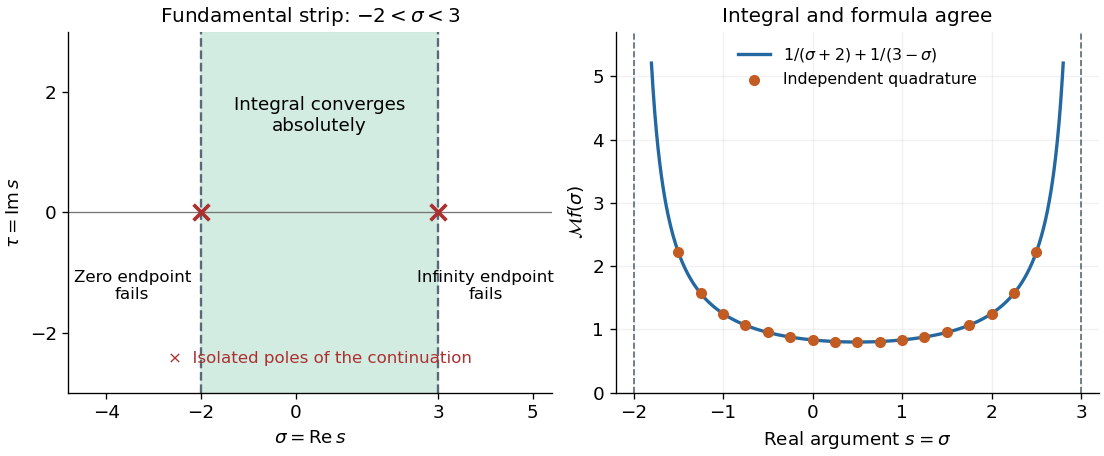
Two endpoint conditions define the Mellin fundamental strip
. Left: the Mellin fundamental strip for below one and above one is . Crosses mark the two poles of the continued rational function, not whole lines of isolated singularities. Right: the formula and independently computed integrals agree on the real slice inside the strip. The curve is drawn only where the defining integral converges. Details.
For , let . Whenever the Mellin transform of is absolutely convergent,The Mellin fundamental strip is unchanged: the corresponding integrals of absolute values differ by the finite positive factor . The change of variables gives , proving the rule. For , the transform's absolute value changes by , while the factor changes its phase. On the line , wherever absolute convergence holds, the transform's absolute value is preserved.
For the Mellin transform of an interval indicator, replacing by givesAt the removable singularity , both sides have value . Scaling leaves the width measured by the natural logarithm unchanged. Likewise, the exponential function has Mellin transform on .
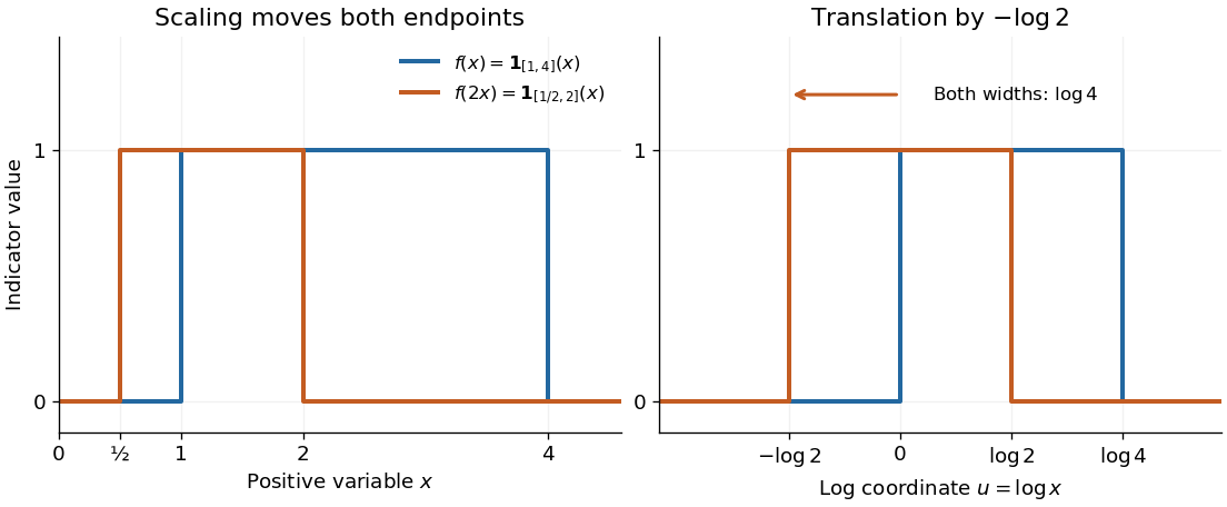
Scaling a positive variable translates its logarithmic coordinate
. Left: moves the support interval to . Right: turns the same change into a translation to the left by ; the interval width remains . The scaling property of the Mellin transform multiplies the transform by . Details.
The change of variables , using the exponential function, turns the Mellin transform intoThe factor changes to ; missing this factor would shift every exponent by one. With and the Fourier transform convention , the identity isChoosing inside the Mellin fundamental strip makes a Lebesgue integrable function. The minus sign in the Fourier transform argument follows from the stated convention. For the Mellin transform of an interval indicator with and , : the Fourier transform of an interval indicator is literally the same computation in a different coordinate.
Splitting the real line at also connects the Mellin transform to two unilateral Laplace transforms. If and for , thenwhere both integrals converge absolutely. Their Laplace convergence regions impose opposite endpoint conditions, explaining the two sides of the Mellin fundamental strip. Finally, shows that a change of scale is a translation in . Weighted Fourier transforms of this translation give exactly the factor in the scaling property of the Mellin transform. For a smooth function with compact support inside , the Mellin inversion theorem follows from Fourier inversion; the existing formula states the corresponding hypotheses.
At exponent zero the complex integral fails absolute and ordinary convergence through its real part, proportional to . The imaginary-part kernel displayed above instead decays as and is integrable. Thus a positive-exponent family can have a well-defined imaginary-part boundary limit even when its full complex limit is invalid. Endpoint expansion coefficients need not be uniform in that limiting exponent: a sine zero can cancel a gamma-function pole and introduce a new nonzero constant term.
Suppose decays faster than every power at infinity and, near zero, for every , with strictly increasing and tending to infinity. Subtracting finitely many terms in the integral over givesThe last integral is holomorphic on . These expressions continue the Mellin transform meromorphically to the whole plane, with simple poles precisely at for nonzero .
Strict increase alone does not suffice in the preceding theorem. Let , and , where is continuous, equals one on and vanishes on . After division by the next power, every finite remainder extends continuously to zero. Nevertheless the Mellin transform has genuine poles at accumulating at , so it cannot be a meromorphic function on the whole plane.
Under standard decay and regularity hypotheses,If is smooth and compactly supported in , its Mellin transform is entire, decays faster than every power on vertical lines, and the formula holds for every real and every .
The unilateral Laplace transform of a function is the integral transformHere is a complex number, is its real part, and is the imaginary unit. The exponential function factor weights the history, while probes its oscillations. The integral starts at zero, so it uses only the history from that starting time onward. This section concerns ordinary functions; their value at the single endpoint does not change the integral. See MIT 18.03SC, definition and elementary examples.
The Laplace transform is useful because it packages an entire time history into a function of : a derivative becomes multiplication by together with the initial value, and a convolution becomes a product. Thus a linear differential equation can become an algebraic equation that already remembers its initial value problem. The worked example below shows both descriptions of the same response.
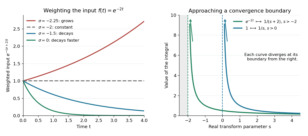
If is a piecewise continuous function and has exponential order , then its defining integral is absolutely convergent for . This is a sufficient condition; the actual Laplace convergence region may be larger than the bound obtained from a chosen . [ref]
https://ocw.mit.edu/courses/18-03sc-differential-equations-fall-2011/fff4420903d82c5c5c483e54566bc5ec_MIT18_03SCF11_s27_2text.pdf. MIT 18.03SC, domain and growth conditions
.

The bound has a short explanation. For sufficiently large , , so , whose tail integral is finite for . The finite initial interval is covered by piecewise continuity.
Three calculations make the convergence condition concrete. For the input , evaluate the finite-history integral first:At the finite-history integral is . For the exponential function input , the same calculation replaces by , givingIn particular, is allowed for this decaying input: its weighted integral is . For the sine input, Euler's formula gives ; linearity then yieldsThe Laplace convergence region is part of the answer. For example, has an analytic continuation to , but the defining integral for the input diverges there. The sine calculation is also developed in MIT 18.03SC, further elementary transforms.
To see why the initial value appears, suppose is an absolutely continuous function on every finite interval , with its right one-sided limit. At the chosen , assume and are Lebesgue integrable functions and . The Laplace transform of a derivative is thenFor example, exponential order bounds on both and guarantee these conditions whenever exceeds both growth bounds. The initial value is the lower-end boundary contribution of integration by parts.
Consider the initial value problemWrite . The Laplace transform of a derivative and linearity give for . A partial fraction decomposition therefore givesWe recognize the two elementary Laplace transforms already computed. Directly verify the result: its derivative is , soThis verifies both the ordinary differential equation and the initial value, and shows that the resulting bounded function has the Laplace transform used above. The response rises from zero toward : at that value the input balances the term . The general method is described in MIT 18.03SC, solving initial value problems.
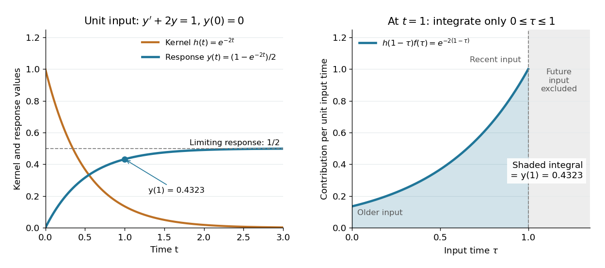

The same solution is a convolution. For functions defined on , the unilateral convolution isThe main convolution article integrates over the whole real line; applying a causal extension by zero to both functions makes its formula identical to this one. Nonzero contributions require both and , hence . If and are Lebesgue integrable functions on , the convolution theorem for Laplace transforms statesFor piecewise continuous functions of exponential order and , it holds throughout . The weighted absolute double integral factors into the two finite weighted absolute integrals; Fubini's theorem therefore permits exchanging the order, and setting separates the product. [ref]
https://ocw.mit.edu/courses/18-03sc-differential-equations-fall-2011/0d4d90053f2bb24f7551c78e2d1b21a2_MIT18_03SCF11_s30_5text.pdf. MIT 18.03SC, convolution and system response
.For the linear time-invariant system starting at zero, the convolution kernel is its impulse response for , extended by zero for . With the Heaviside step function input, for , the accumulated response isThus on is both the algebraic solution and the Laplace transform of a finite-history convolution. Each past input contributes an exponential function that decays with its age , which makes the two descriptions easy to connect.
Finally, compare the Fourier transform convention . If is the causal extension by zero of , define . Whenever is a Lebesgue integrable function,A vertical slice of the Laplace transform is therefore the Fourier transform of the zero-extended, weighted input. Positive damps its positive-time history. A finite window function instead gives and ; this approaches in the Laplace convergence region. Setting directly requires an integrable zero-extended input: the input fails that condition, even though its Laplace transform exists for every .
The history of the Laplace transform spans several stages. Schiff's historical summary notes that Laplace's 1812 treatise acknowledged earlier work on integral transforms and describes later development of the modern Laplace transform method. [ref]
https://oldversion.stu.edu.vn/uploads/documents/170509-091205.pdf#page=9. Schiff, The Laplace Transform: Theory and Applications, historical summary, pp. x–xi
.A function has exponential order if some and give the displayed bound. Bounded functions, including sine, have exponential order zero; has exponential order . The bound need not use the smallest possible . Together with piecewise continuity, it guarantees a Laplace transform for .
The set of complex numbers for which the displayed integral is finite is the region of absolute convergence of a Laplace transform. It depends only on the real part . Once the condition holds for one , it holds for every larger real part. For the exponential function it is exactly ; in general, convergence on the boundary must be checked separately. An analytic continuation outside this set need not equal a convergent defining integral.
Extend a function given for nonnegative time to the real line by setting it to zero before the starting time. This turns unilateral convolution into whole-line convolution and identifies a Laplace transform slice with a Fourier transform after exponential function weighting.
For , this Laplace transform converges at zero because is integrable, and at infinity because of exponential damping. Its large- behavior is governed by a logarithmic zero-endpoint singularity and begins with , rather than a power of .
The Gamma reflection formula gives , analytic at zero with value one. A finite-parameter Watson's lemma representation of Ramanujan's function therefore gives the displayed coefficients. In particular , and , with Euler's constant. Obtaining this representation requires taking an imaginary part before sending its Mellin exponent to zero; the original complex integral is divergent at that boundary.
For bounded locally integrable on the nonnegative real line, suppose its Laplace transform extends holomorphically to an open neighborhood of the closed right half-plane. Then the ordinary improper integral converges to . Contour damping for bounded Laplace transforms bounds the difference from the finite-interval transform by in the limit for every radius . Extension merely to the open right half-plane is insufficient, as the constant function and transform show.
The displayed kernel has residue one at zero and vanishes at the endpoints of a radius- imaginary-axis segment. On either radius- semicircle, , cancelling the inverse real-part bound on a bounded function's Laplace transform tail. Use the full transform only on a right semicircle and a thin analytic leftward path; deform the finite-interval entire transform to the large left semicircle. This proves the Newman Tauberian theorem without assuming analytic continuation across an entire left half-disk.
For functions on with and Lebesgue integrable functions, their unilateral convolution, defined almost everywhere if necessary, satisfiesTaking a causal extension by zero of both functions gives the existing whole-line convolution definition. Absolute convergence and Fubini's theorem justify the product rule: put in the double integral, so . For piecewise continuous functions of exponential order and , the hypotheses hold for . The Laplace transform article works out the concrete example and the Heaviside step function input, whose output is . [ref]
https://ocw.mit.edu/courses/18-03sc-differential-equations-fall-2011/0d4d90053f2bb24f7551c78e2d1b21a2_MIT18_03SCF11_s30_5text.pdf. MIT 18.03SC, convolution and system response
.Under suitable regularity and growth conditions, a function with Laplace transform is recovered by the inverse contour integralwhere the vertical line lies to the right of every singularity of .
A Laplace transform can grow exponentially as . At an evaluation time , multiplying by does not automatically permit closing the inverse contour to the left. Either retain the growth-bearing contour pieces, use a causal time convolution, or justify a deformation with the time-truncated transform. Resolvent-pole information alone is insufficient.
Terms singular at in a Laplace transform encode persistent late-time behaviour. In particular,contributes to the inverse transform; singularities farther into the left half-plane contribute decaying terms under the usual analyticity and growth assumptions.
Suppose is an absolutely continuous function on every finite interval , both and are Lebesgue integrable functions, and . Then integration by parts on followed by a limit givesHere is the right one-sided limit. Exponential order bounds on and suffice when exceeds both bounds. For , the identity reads on . This is the ordinary derivative on nonnegative time; differentiating a causal extension by zero at its jump instead introduces a Dirac delta function. [ref].
For , .
The delayed unit step has
The Heaviside function is zero before its switching time and one after it, allowing delayed signals to be written algebraically.
Articles by others on the same topic
There are currently no matching articles.