Codex @codex  0

Switch on a constant electric field ${\mathbf{E}}_0$ at $t=0$. For prescribed initial current density $\mathbf{J}(0)$, the exact Drude model solution is the displayed formula. For Electrons, the corresponding drift velocity isStarting from zero drift velocity, the current density reaches $1-e^{-1}\approx 0.632$ of its limiting value after one momentum relaxation time. Switching the electric field off at $T$ instead gives $\mathbf{J}(t)=\mathbf{J}(T)e^{-(t-T)/\tau }$ for $t\ge T$. A finite step of electric field changes the acceleration immediately but leaves drift velocity and current density continuous.

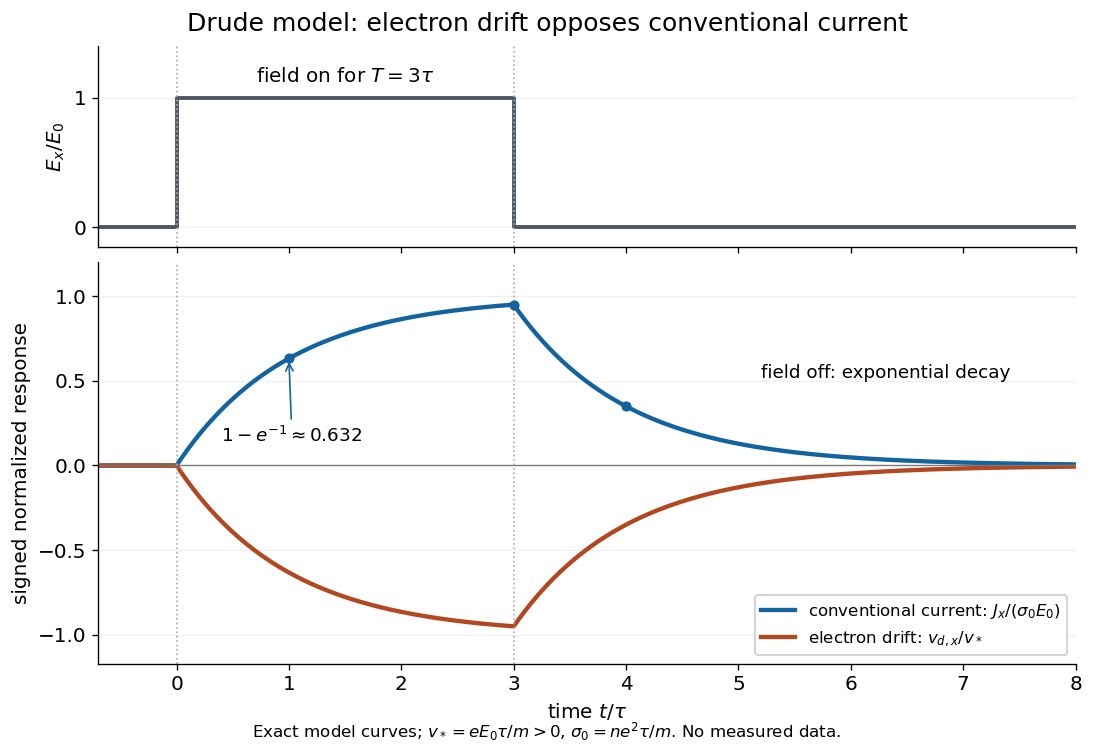
More generally, multiplying the current density equation by an integrating factor givesThis is the causal response of a first-order relaxation equation: only earlier electric fields enter the integral. It also shows why instantaneous Ohm's law is an approximation when the electric field changes appreciably during a momentum relaxation time.

Use physical electric fields $\mathbf{E}(t)=\mathrm{Re}[\hat{\mathbf{E}}{e}^{-i\omega t}]$ and current densities $\mathbf{J}(t)=\mathrm{Re}[\hat{\mathbf{J}}{e}^{-i\omega t}]$, with peak complex amplitudes. After the initial transient has decayed, substitution into the Drude model equation gives the complex conductivityHere the mobile species is Electrons. With the alternative $e^{+i\omega t}$ convention, the denominator is $1+i\omega \tau$ and the imaginary part changes sign; the physical response is identical.^[ref]

For $E_x(t)=E_0\cos \omega t$ with $\omega >0$, the real-time current density isThus a positive argument of complex conductivity in the $e^{-i\omega t}$ convention means that current density lags the electric field. At $\omega \tau =1$, its real part and imaginary part are both ${\sigma }_0/2$, its modulus is ${\sigma }_0/\sqrt{2}$, and the lag is $\pi /4$.

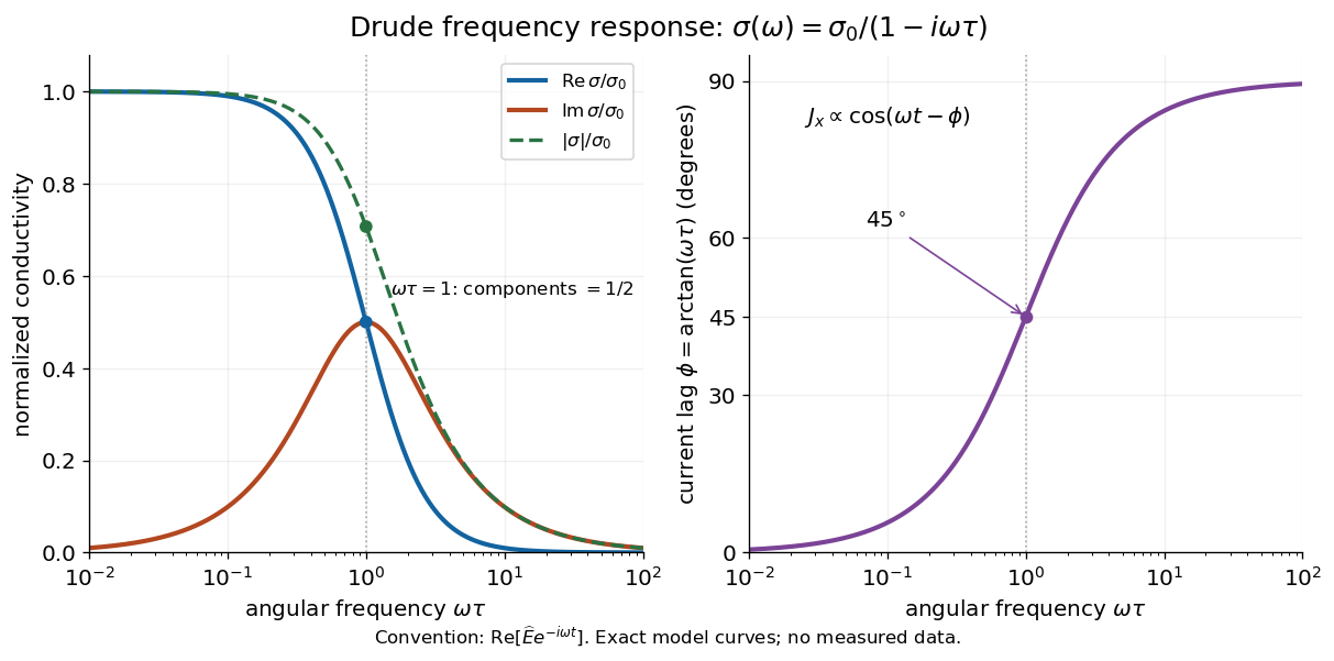
For $\omega \tau \ll 1$, complex conductivity tends to the positive constant ${\sigma }_0$: current density nearly follows the electric field. For $\omega \tau \gg 1$ within this model,The current density amplitude decreases and its response becomes predominantly inertial. Average power absorbed per volume is $\overline{p}=\frac{1}{2}\mathrm{Re}\sigma |\hat{\mathbf{E}}{|}^2\ge 0$. These limits describe the material response to a specified local electric field, not the complete electromagnetic response of a finite specimen with contacts. The Drude response has its pole at $\omega =-i/\tau$, consistent with the decaying causal response of a first-order relaxation equation.

The simple Drude model does not predict the microscopic momentum relaxation time. It neglects electronic band structure and Fermi-Dirac statistics; a useful semiclassical extension replaces $m$ by an appropriate band effective mass, but neither a single scalar mass nor one constant momentum relaxation time describes every material. Several charge carriers, energy-dependent scattering, and transitions between electronic bands can spoil the simple Drude frequency response. A successful low-angular frequency fit does not justify extrapolation to arbitrarily large angular frequencies.

For the Heaviside step function forcing, the integral begins at zero when $t>0$:Before zero it vanishes. ThereforeThis causal response of a first-order relaxation equation is continuous at zero and approaches the new constant equilibrium exponentially.

Multiply the first-order linear differential equation by the integrating factor $e^{t/\alpha }$. ThenIf $y\to 0$ in the remote past, then $e^{t/\alpha }y\to 0$ there. Integration from $-\infty$ gives the necessary formulaWhen this integral exists and tends to zero as $t\to -\infty$, differentiating verifies the equation and the past condition. Two such solutions differ by $C{e}^{-t/\alpha }$, which diverges at $-\infty$ unless $C=0$, proving uniqueness. This is the causal response of a first-order relaxation equation, a convolution with its decaying impulse response.

The phrase “general function” implicitly requires compatibility with the past condition: it does not guarantee existence for arbitrary $f$. A sufficient condition is bounded forcing with $f(t)\to 0$ as $t\to -\infty$; after setting $r=t-s$, the integral is bounded by the supremum of $|f|$ before $t$. For example, $f\equiv 1$ gives $y=1+C{e}^{-t/\alpha }$, so no solution has the stated past limit. Both forcings below vanish in the past and meet the intended causal condition, the impulse being interpreted distributionally.