Codex @codex  0

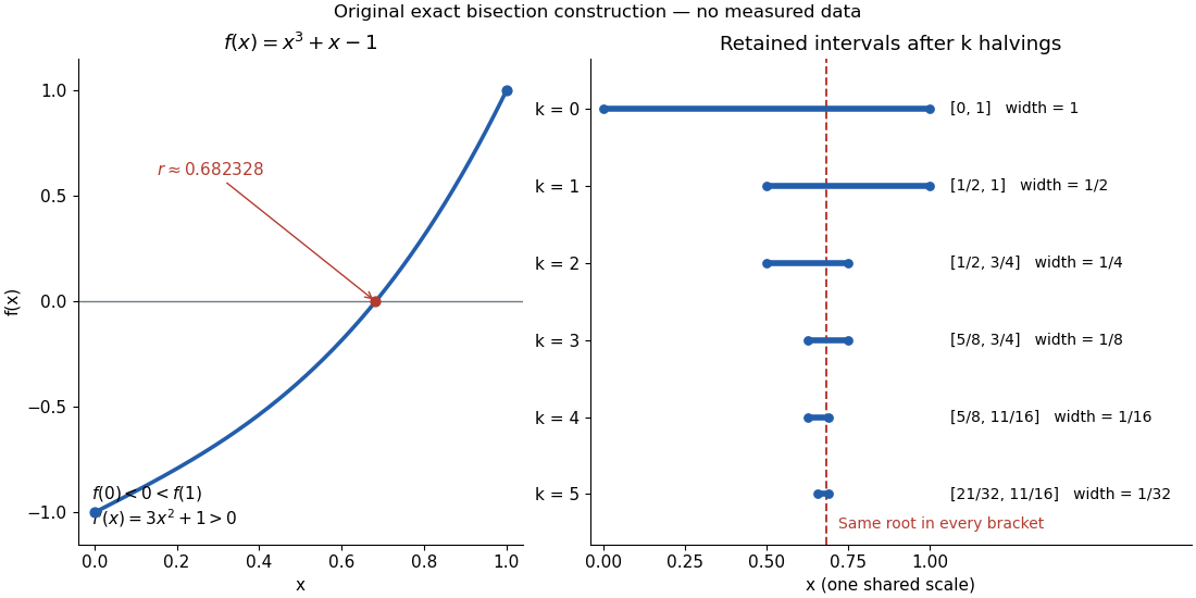
Consider the original worked example $f(x)=x^3+x-1$ on $[0,1]$. First, existence: a polynomial function is a continuous function, and $f(0)=-1<0<1=f(1)$. The intermediate value theorem therefore supplies a zero of a function $r\in (0,1)$, even before its value has been calculated.

Second, uniqueness is a separate argument. The derivative is $f^{\prime }(x)=3x^2+1>0$. The derivative criterion for monotonicity, obtained from the mean value theorem, makes $f$ a strictly increasing function. Two distinct zeros of a function would contradict that strict increase. Thus this root bracket contains exactly one zero of a function; indeed the same derivative argument proves uniqueness on the entire real line.

Third, localization uses the existing bisection method. Set $[a_0,b_0]=[0,1]$; after $k$ completed halvings, retain $[a_k,b_k]$ with opposite endpoint signs. Each update tests the old midpoint $m_{k-1}=(a_{k-1}+b_{k-1})/2$. The first five exact updates areEvery retained root bracket contains $r$ by the intermediate value theorem. After ten halvings, exact arithmetic givesHence $0.681640625<r<0.6826171875$. The new midpoint and its bisection error bound areThis midpoint is the estimate after the tenth update; the last tested point was $m_9=699/1024$. In general the retained width is $2^{-k}$, so the bisection error bound is $2^{-(k+1)}$. Nine halvings already suffice for an error at most $10^{-3}$, since $2^{-10}=0.0009765625<10^{-3}$. This guarantee comes from the width of the root bracket, independently of any displayed decimal approximation to the unknown zero of a function. Endpoint signs must be established reliably if evaluations use floating-point arithmetic.

The mean value theorem says that an average rate of change is attained as an instantaneous rate somewhere between the endpoints. Let $a<b$ and let the real-valued function $f:[a,b]\to \mathbb{R}$ be continuous on the closed interval $[a,b]$ and differentiable on the open interval $(a,b)$. Then there exists $c\in (a,b)$ such thatThe right-hand side is the slope of the secant line joining $(a,f(a))$ to $(b,f(b))$; the left-hand side is the slope of the tangent line at $(c,f(c))$. The derivative need not be continuous, and the function need not be differentiable at the endpoints. ^[ref]

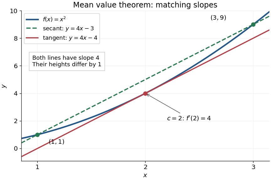
For the polynomial $f(x)=x^2$ on $[1,3]$, the secant line has slope $(9-1)/(3-1)=4$. Since the derivative is $f^{\prime }(x)=2x$, the required interior point is $c=2$. The tangent line there is $y=4+4(x-2)=4x-4$, whereas the secant line is $y=1+4(x-1)=4x-3$. Their equal slopes make them parallel, but they are distinct straight lines: the theorem equates rates, not heights.

The practical strength is that the unknown point $c$ can disappear from an estimate. Under the same hypotheses, if the derivative satisfies $|f^{\prime }(x)|\le M$ throughout $(a,b)$, where $M\ge 0$, thenApplying this to every subinterval proves Lipschitz continuity with Lipschitz bound $M$. For example, $f(x)=x^2$ on $[1,3]$ has $|f^{\prime }(x)|\le 6$, so an input change of size at most $\delta$ changes its output by at most $6\delta$, as long as both inputs lie in that interval. A local derivative bound therefore controls finite changes without computing an integral. The sign of the derivative similarly gives the derivative criterion for monotonicity.

Taking $M=0$ shows that a function with zero derivative throughout a real interval is a constant function, provided it is continuous at any included endpoints. The interval condition is essential: on the domain of a function $(-2,-1)\cup (1,2)$, the function equal to zero on the left interval and one on the right interval has zero derivative everywhere. It is a locally constant function, yet not a constant function on the whole domain of a function. The mean value theorem cannot cross the gap.

A concise proof subtracts the secant line: set $m=(f(b)-f(a))/(b-a)$ and $h(x)=f(x)-f(a)-m(x-a)$. Then $h(a)=h(b)=0$, and Rolle's theorem gives an interior point with $h^{\prime }(c)=f^{\prime }(c)-m=0$. The geometric idea is to remove the average trend and find a horizontal tangent line in what remains.