Epsilon-delta definition of continuity ($\forall \epsilon >0\exists \delta >0$)

A function $f:D\to \mathbb{R}$ is continuous at $a\in D$ whenFirst choose the required output tolerance $\epsilon$; then choose an input tolerance $\delta$ that works for every allowed function input in that window. Picking a different $\delta$ separately after seeing each $x$ would reverse the quantifiers and lose this guarantee. There is no need to exclude $x=a$, because the output difference is then zero.

At an isolated point of the domain of a function, choose a small enough window that its only allowed function input is $a$. This proves continuity there directly. At a point with arbitrarily close other inputs, the same definition is the limit of a function condition $f(x)\to f(a)$. For metric spaces, replace the two absolute values by their distance functions; for arbitrary topological spaces, the corresponding definition is a continuous map.

The input tolerance may depend on $a$. A single choice valid everywhere on the domain of a function is the stronger requirement of uniform continuity. The continuous function $x\mapsto x^2$ on $\mathbb{R}$ shows the difference: for any proposed $\delta >0$, the points $a=1/\delta$ and $b=a+\delta /2$ have $|b-a|<\delta$, yet $b^2-a^2=1+{\delta }^2/4>1$. Thus the fixed output tolerance $\epsilon =1$ admits no global input tolerance on the real line.

For $f(x)=x^2$ at any real $a$, polynomial factorization givesIf $|x-a|<1$, the triangle inequality yields $|x+a|\le |x-a|+2|a|<2|a|+1$. Therefore the displayed choice of $\delta$ makes $|x-a|<\delta$ imply $|f(x)-f(a)|<\epsilon$. This proves continuity and gives an explicit local error bound, rather than an inference from a drawing.

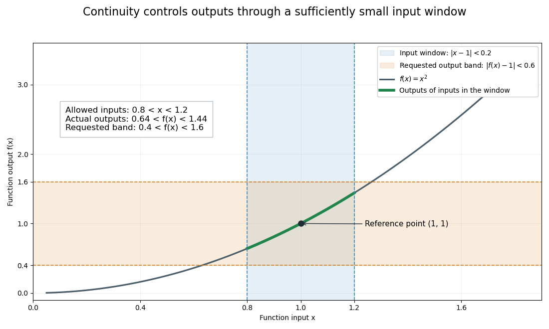
At $a=1$ and $\epsilon =0.6$, this sufficient choice is $\delta =0.2$. The permitted function inputs satisfy $0.8<x<1.2$; their actual function outputs lie in $(0.64,1.44)$, inside the requested band $(0.4,1.6)$. A sufficient input window need not be the largest possible one.