Real analysis studies limits, continuity, differentiation, integration, and convergence of sequences and functions taking values in the real numbers. Its central question is how finite approximations determine an exact answer: what does an arbitrarily small error mean, and which operations respect that error? A derivative is a limit of quotients, while a Riemann integral is obtained from increasingly fine Riemann sums. Both need conditions that make the answer independent of the approximations chosen.
Two organizing ideas are completeness of the real numbers, which ensures that suitable approximations have a destination, and uniform convergence, which controls approximation error over an entire domain. Pointwise convergence supplies separate guarantees at separate inputs; uniform convergence supplies one guarantee for all inputs. This distinction explains why replacing an approximating function by its limit can preserve continuity or integrals under appropriate hypotheses, yet fail without them.
For historical context, Cauchy's 1821 Cours d'analyse explicitly discusses convergence of series. Its Note VII treats double series and compares summing by rows and by columns under stated convergence assumptions: controlling an infinite process was already a concrete problem. This is historical context for questions about limits, rather than an attribution of the modern definitions below. [ref]
https://www.e-rara.ch/download/pdf/8543076.pdf. Cauchy, Cours d'analyse (1821), Note VII, pp. 537–539, original scan
. The initial table of content was limited to the first level because it is larger than 1000 articles. There are 1015 articles in total. Expand a branch to load its children.
Hardy's inequality bounds averages or weighted functions by their original size or derivatives. For and , its integral form is . Spatial weighted forms include the Hardy inequality in Euclidean space.
Let and let be a real or complex measurable function in Lp space , with Lebesgue measure . The Hardy operator, denoted here by , takes the running averageHölder's inequality ensures , so every such average exists. Hardy's integral inequality statesThe real signed and complex extensions of the nonnegative statement follow from the triangle inequality . Changing on a null set changes neither average nor Lp norm.[ref]
Inequalities by Godfrey Harold Hardy and others. Inequalities, second edition, §9.8, Theorem 327, equation (9.8.2), printed p. 240
Averaging over an expanding interval spreads a localized input across the whole positive half-line. Hardy's integral inequality bounds the total Lp norm of that spread. The Hardy operator is consequently a bounded linear operator on this Lp space. The factor bounds its operator norm; its th power is the constant in the displayed integral bound. These are different constants: at , the L2 norm bound is two and the squared L2 norm bound is four.
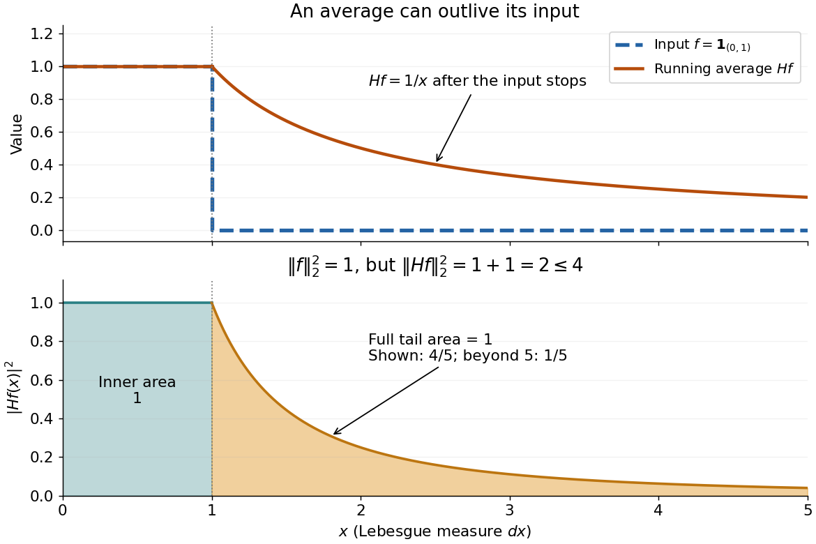
Take the indicator function . Direct integration givesAlthough the function vanishes beyond one, its average remembers the unit area accumulated before one. Squaring and integrating both portions givesThus the tail accounts for half of the squared L2 norm. Averaging does not always decrease the L2 norm with this Lebesgue measure on the half-line. The same indicator function also explains the restriction : , so its average is not in L1 space.
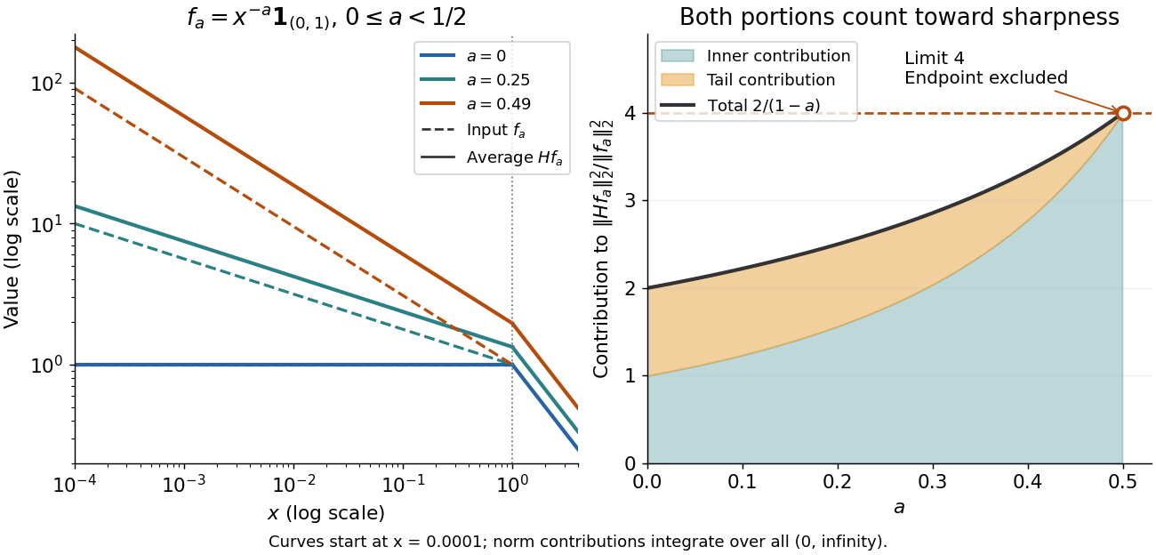
The indicator function example reaches a squared L2 norm ratio of two. To approach four, concentrate more strongly near zero. For , use the measurable functionAll integrals use Lebesgue measure . Keeping both portions of the squared L2 norm givesConsequently,Every allowed member has ratio strictly below four. For any proposed constant , a sufficiently large has ratio greater than . Combined with Hardy's integral inequality, this proves that four is the smallest possible squared L2 norm constant.[ref]
Inequalities by Godfrey Harold Hardy and others. Inequalities, second edition, §9.8, Theorem 327, printed p. 240, and sharpness argument on printed p. 243
The endpoint is excluded: at , , and the inner portion of also diverges. Its tail still has finite integral four. There is no finite L2 norm ratio at this endpoint, hence no equality example obtained by substituting it. The limit four is unattained by this family. Multiplying each by makes its L2 norm one without changing the ratio.
For a nonnegative , first set and . These bounded functions vanish near zero and have compact support. Their averages have finite Lp norms: they vanish near zero and decay as beyond . Integration by parts givesThe boundary term vanishes at zero because is zero there, and at infinity because is eventually constant and . The inequality is Hölder's inequality with conjugate exponents and . Divide when ; the zero case is immediate. Since and , the monotone convergence theorem proves the full bound without presupposing that has finite Lp norm. Apply it to for the signed or complex case.[ref]
Inequalities by Godfrey Harold Hardy and others. Inequalities, second edition, §9.8(ii), truncation and integration by parts, printed pp. 242–243
For a subset of a partially ordered set, its infimum is its greatest lower bound and its supremum is its least upper bound. An upper bound only has to lie above every member; the supremum is the smallest such bound. A lower bound lies below every member; the infimum is the largest such bound. These definitions identify the exact edges of a set even when neither edge belongs to it.
For example, and both have infimum zero and supremum one. Only has a minimum and a maximum: those must be actual members of the set. The set has infimum zero without a minimum, but its supremum one is also its maximum. Such examples distinguish a bound from an attained extremal value. [ref].
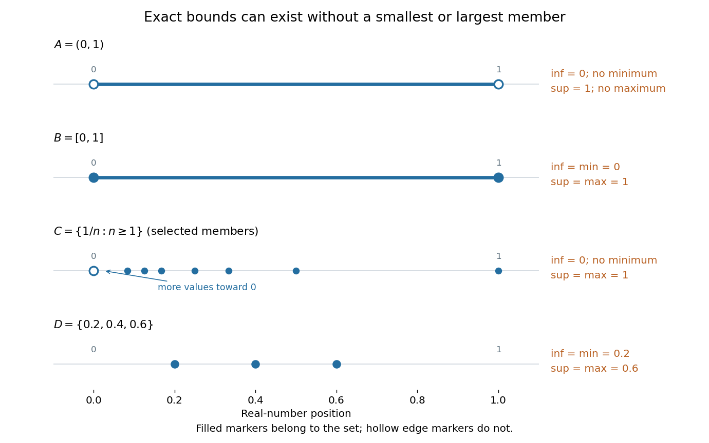
For a nonempty subset of the real numbers, completeness of the real numbers guarantees a real supremum when it is bounded above, and a real infimum when it is bounded below. The bound and the ambient partially ordered set both matter: has supremum in the real numbers, but no supremum in the rational numbers. The detailed explanation belongs to completeness of the real numbers.
Why are unattained bounds useful? They specify a precise limiting target. In mathematical optimization, on has infimum zero but no global minimizer. The inputs for give a minimizing sequence: their objective values approach zero without ever reaching it. Bounds therefore describe what approximation can achieve even when no feasible input is best. The approximation property of an infimum and approximation property of a supremum express this idea quantitatively.
The essential infimum and essential supremum describe the lower and upper bounds of a measurable function after disregarding null sets for a specified measure. A pointwise infimum or supremum sees every input; an essential bound sees whether values below or above a proposed threshold occur on a set of positive measure. Thus "essential" means insensitive to changes on a null set, rather than insensitive to unusual values. This distinction makes essential bounds compatible with Lebesgue integrals and the equivalence classes used in Lp spaces. [ref]
Lp spaces (Chapter 7 of Measure Theory). Hunter, Measure Theory, Definitions 7.1, 7.3–7.4: almost-everywhere equivalence and essential bounds
.For a real measurable function on a measure space , the definitions areThese can take values in the extended real number line. On a space of positive total measure, finite essential bounds obey almost everywhere. If is finite, every threshold has ; the corresponding lower-edge statement is for every . These are the measure-based counterparts of the approximation property of a supremum and approximation property of an infimum.
Here is a two-sided example on with Lebesgue measure:The pointwise bounds are and , while the essential bounds are and . Both exceptional singletons are null sets. But for , the inputs where still have measure , and those where have measure : deleting or adding two individual inputs cannot change those lengths. Hence neither essential bound can be moved inward.
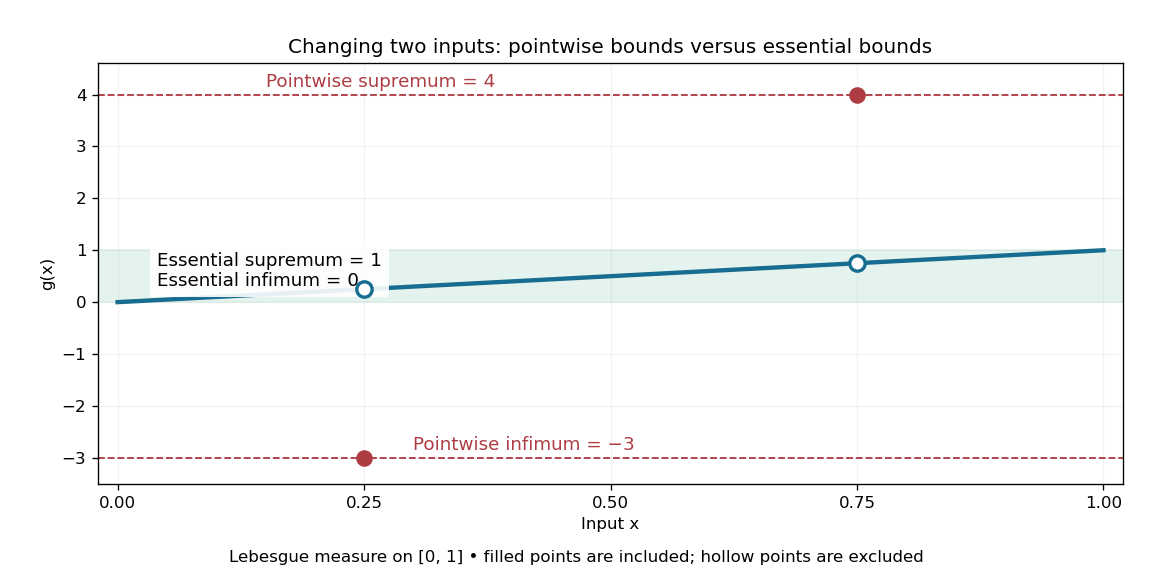
Essential infimum and essential supremum ignore two exceptional singletons, while pointwise infimum and supremum retain them
. The function follows except for the filled values and . Hollow markers exclude the ordinary values at those inputs. The shaded horizontal band spans the essential bounds zero and one for Lebesgue measure. Details.The choice of measure is part of the answer. The same has essential bounds and under counting measure, because every nonempty set has positive measure. Under the Dirac measure at , both essential bounds equal . A null set for one measure need not be a null set for another.
Nor must the exceptional inputs be isolated. The Dirichlet function, equal to one at rational numbers and zero at irrational numbers, has pointwise supremum one on , but essential supremum zero for Lebesgue measure: the rational numbers form a countable set that is a null set, even though they are dense. Conversely, a value ten on an interval of length affects the essential supremum just as decisively as it would on half the domain. Small positive measure is not zero measure.
The essential infimum of a real measurable function is . It is the largest lower bound that holds almost everywhere, with values allowed in the extended real number line. Unlike a pointwise infimum, it is unchanged by altering a representative on a null set.
For the function in essential infimum and essential supremum, the value at one input changes the pointwise infimum, but the essential infimum remains zero under Lebesgue measure. If instead a function is throughout an interval of any positive length and zero elsewhere, its essential infimum is . The distinction concerns the measure of the low-value set, rather than the magnitude of the low value.
For a nonempty set , a real number is its supremum precisely when it is an upper bound and no smaller real number is an upper bound. It is unique: two least upper bounds must each be no greater than the other.
For , every number at least one is an upper bound, and none smaller than one bounds the whole set. Thus , although . For , that same supremum is also the maximum. The approximation property of a supremum supplies witnesses arbitrarily close to an unattained upper edge.
Let be nonempty and bounded above. An upper bound equals exactly when, for every , some satisfies . If no such member existed, would be a smaller upper bound. Conversely, the condition defeats every proposed upper bound by taking . [ref].
For and , is one witness: . Choosing with produces a sequence converging to by the squeeze theorem. The choices need not form a monotone sequence.
If a nonempty real set has finite supremum and , then every interval contains infinitely many elements of . Otherwise its finitely many elements have a largest value ; all remaining elements are at most , making an upper bound. The interval cannot be empty either, by the defining approximation property of a supremum. Thus failure to attain a finite supremum forces accumulation from below.
For a nonempty set , a real number is its infimum precisely when it is a lower bound and every other lower bound is at most . It is the greatest lower bound, not necessarily the minimum.
For , zero is a lower bound. Every positive candidate fails: the Archimedean property gives an integer , hence . Thus , although zero is never a member of . This is the lower-edge counterpart of approximating an unattained supremum.
Let be nonempty and bounded below. A lower bound equals exactly when every admits with . Otherwise would be a larger lower bound. Taking tolerances gives a sequence of members converging to . For a real-valued objective with finite infimum, this supplies a minimizing sequence without assuming that a global minimizer exists.
Asymptotic analysis describes what remains dominant as an argument approaches a specified limit. It compares functions or sequences by scale: how much of a complicated expression can be replaced by a simpler one, and how large is the omitted part? The limit may be for a growing input or for a shrinking approximation parameter.
For example, is eventually dominated by its quadratic term, since division by gives . But at , the linear term contributes , compared with only from the quadratic term. A statement about the limiting scale and a good approximation at a particular input are different claims.
Three useful comparisons keep their strengths distinct. Big O notation supplies an eventual upper bound up to a constant multiplier; big theta notation supplies both an upper bound and a lower bound up to constants; asymptotic equivalence makes the ratio tend to one. Little o notation says that a term becomes negligible relative to a specified scale. These distinctions make approximations checkable instead of merely calling one expression small.
The same language connects time complexity with Taylor remainders. In an operation-count model, one asks how a cost scales with input size. In a Taylor expansion, one asks how the approximation error scales with the increment. Neither use requires interpreting the unspecified constant as one. The asymptotic comparison of exponential functions gives another example: dividing by the largest contributing exponential reveals the terms that disappear.
For functions with nonzero sufficiently near a specified limit,The same definition applies to sequences as . Equivalently, : replacing by has a relative error tending to zero, and the difference is in little o notation. The limit and reference scale are essential parts of the statement.
For example, because . Replacing the former by the latter gives absolute error , which grows without bound. Thus asymptotic equivalence controls a ratio, rather than requiring the absolute error to vanish. This distinction is crucial when approximating a rapidly growing factorial with Stirling's formula.
By contrast, and have the same order in big theta notation, but are not asymptotically equivalent: their ratio remains two. For positive functions, asymptotic equivalence gives both-sided constant bounds eventually, whereas constant bounds alone do not recover the leading coefficient.
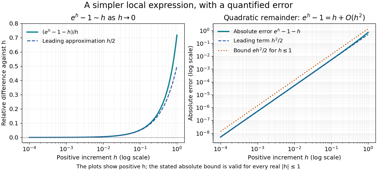
For a local example with real , the exponential function obeys as . The Taylor theorem with Lagrange remainder givesThus for ,This states in big O notation, and division by shows that the relative difference measured against vanishes. The diagram uses positive ; the bound is valid on both sides of zero. At , the absolute error is approximately and the relative difference against is approximately .
For positive bases , comparison of the exponential functions and reduces to a geometric progression:If , this ratio tends to zero, so in little o notation. If , the ratio is one; if , it grows without bound.
Consequently, provided at least one coefficient is nonzero, a finite sum with distinct positive bases is asymptotically equivalent to its largest-base term whose coefficient is nonzero. For example,The relative difference against first drops below one percent at the integer . Dividing by the proposed dominant term provides an explicit error estimate, not just a comparison of two rapidly growing numbers. If several terms have the same largest base, their coefficients must first be combined; cancellation can remove that base entirely.
Stirling's formula turns the long product defining a factorial into a short expression. For positive integers , putThen as . This is asymptotic equivalence: , so the relative error tends to zero. It does not say that the absolute error tends to zero, and the formula is not an equality for finite . The Gamma function extends this approximation beyond integer inputs. [ref]
https://dlmf.nist.gov/5.11. NIST Digital Library of Mathematical Functions, §5.11: Gamma-function asymptotic expansions
For ,The leading estimate is about low. Multiplying by the first correction factor giveswhich is about low. The Stirling correction by Gaussian moments explains why this factor is rather than an arbitrary numerical adjustment.
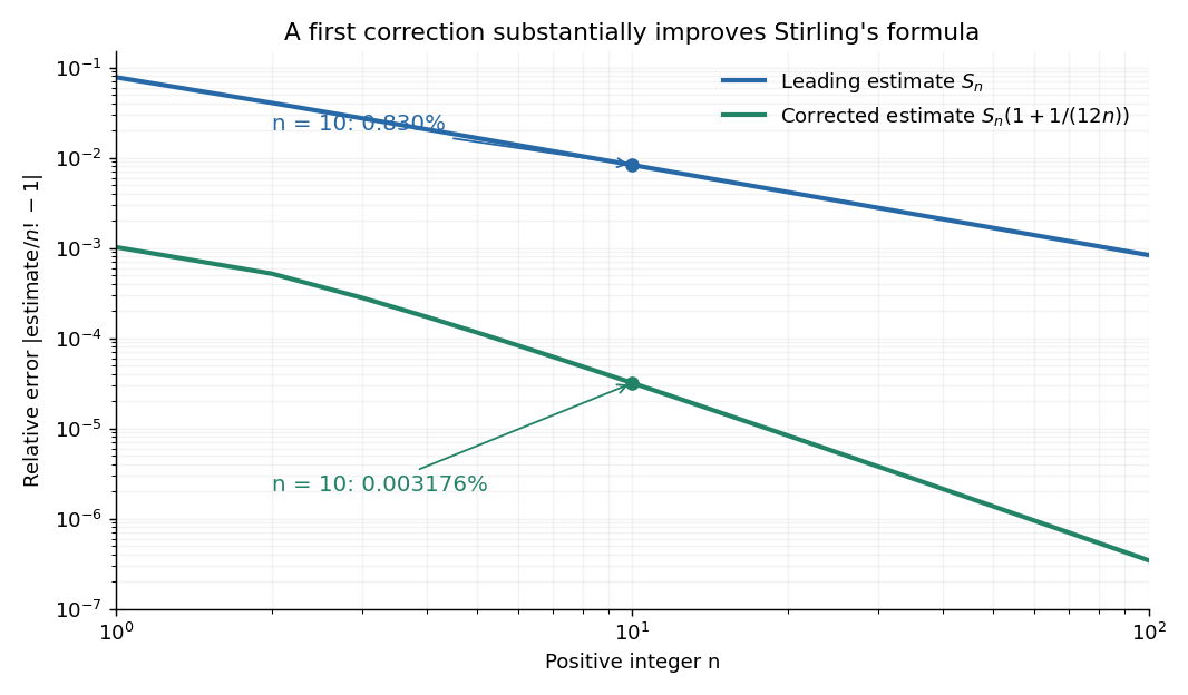
The usefulness is in ratios as well as in enormous numbers. Applying Stirling's formula to the three factorials in a central binomial coefficient givesThis counts the ways to choose exactly half of objects. Equivalently, for independent fair coin tosses, the binomial distribution assigns probability to exactly heads. An exponentially large count becomes a simple probability scale after cancellation.
For numerical calculations, taking the natural logarithm yieldswhere . Computing a logarithm of a large factorial avoids representing the factorial itself. The Robbins bounds for Stirling's formula give a finite- interval for this logarithmic remainder, rather than only a limiting statement.
The factor is beautiful because a Gaussian integral lies behind a discrete product. The Gaussian peak behind Stirling's formula displays this connection through the Gamma integral and Laplace's method. A rigorous proof must also control the tails of the integral; the local expansion explains the geometry but is not by itself a complete proof.
James Stirling published Methodus differentialis in 1730, a treatise on summation and interpolation of infinite series. This setting connects the formula with a practical calculation problem: taking logarithms turns a long product into a sum, whose growth can be approximated. [ref]
https://commons.wikimedia.org/wiki/File:Methodus_differentialis,_sive_tractatus_de_summatione_et_interpolatione_serierum_infinitarum_(IA_10053880bsb).pdf. James Stirling, Methodus differentialis (1730), digitized original and bibliographic record
For every positive integer , Herbert Robbins's bounds giveEquivalently, the remainder in satisfies . This both proves that underestimates and squeezes to one, establishing Stirling's formula. Robbins published the bounds in “A Remark on Stirling's Formula” in 1955. [ref]
https://dornsife.usc.edu/sergey-lototsky/wp-content/uploads/sites/211/2024/02/Stirling-Robbins.pdf. Herbert Robbins, American Mathematical Monthly 62 (1955), pp. 26–29, equations (1)–(2)
For , the relative error of lies strictly between and , approximately and . A bound specifies the accuracy of an approximation before using it in another calculation.
Repeated integration by parts gives the Gamma integralThe logarithm of its integrand is , whose unique maximum is at . Write . For fixed and large , a Taylor expansion givesThe Big O notation here is for a fixed , or uniformly for in a fixed bounded interval. It does not claim a uniform approximation over the entire growing integration domain. Consequently the peak, divided by its height, approaches .
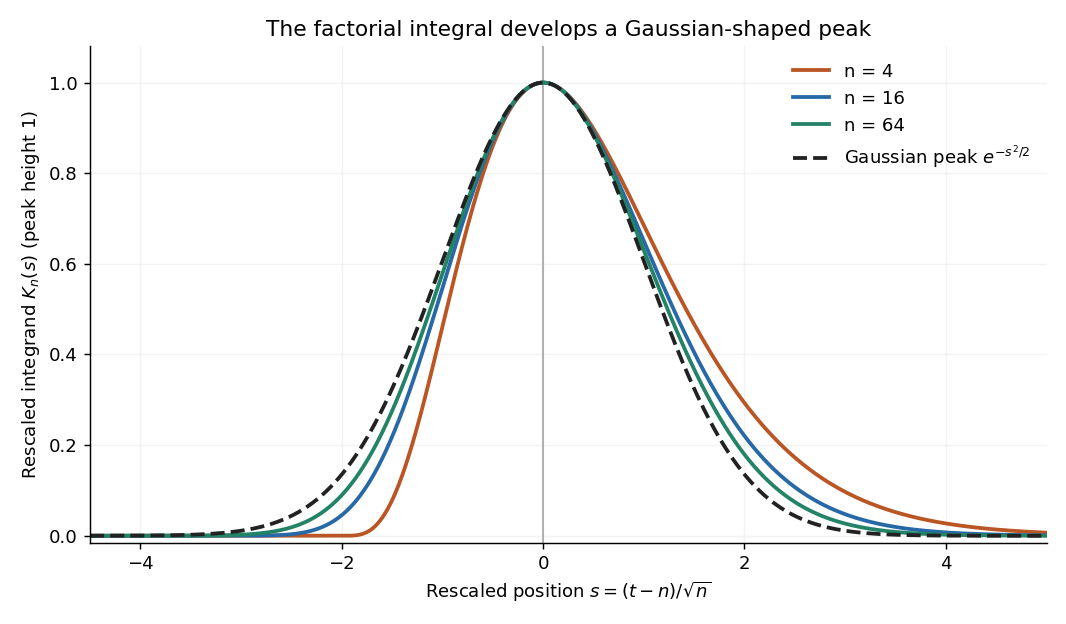
The exact substitution givesReplacing the integral by the Gaussian integral produces . Thus the estimate is peak height times width times the area of a standard Gaussian peak. This is Laplace's method in a concrete form; controlling the integral's tails justifies the replacement. The next terms, including their products after exponentiation, produce the Stirling correction by Gaussian moments.
In Laplace method for the Gamma function, scaling gives a standard Gaussian integral. The first even correction polynomial is . Its expectation under a unit-variance centered Gaussian is . The amplitude expansion contributes to this coefficient as well as the phase expansion; expanding only the latter gives the wrong Stirling formula correction.
For nondecreasing real , convergence of the displayed improper integral forces . For , the integral over tends to zero and is at least . The integral over tends to zero and is at most . These bound the upper and lower limits by and . Letting squeezes both to one. The limit of the improper integral must be finite.
A function is homogeneous of degree when rescaling its arguments by a common scalar rescales its value by , whenever the arguments and that power are defined. For integer over a vector space, one can require every nonzero scalar; a homogeneous polynomial gives an example. On a domain stable under positive real rescaling, the positive-scaling version allows real . Degree-one positive homogeneity is the convention used for norms and many convex functions. The Euler theorem for homogeneous functions turns this scaling law into a differential identity for a differentiable function.
Homogeneity of degree means that multiplying all arguments by a common positive factor multiplies the output by . A homogeneous function is the function possessing this property. This is different from degree-one positive homogeneity; investment values with constant relative risk aversion utility usually have degree .
A function on a cone is positively homogeneous of degree one when for every . If such a function is concave, thenbecause homogeneity rewrites the left-hand side as before concavity is applied.
Let be a differentiable function on an open domain stable under positive rescaling, with for . The chain rule differentiates this homogeneous function identity at to giveIf is twice differentiable, differentiating once more gives . In degree one its Hessian matrix therefore annihilates the radial vector . This is the identity used in the no-scale identity from degree-one homogeneity. For an extensive quantity, the degree-one formula also supplies the thermodynamic identity behind the Gibbs-Duhem equation.
On an open domain invariant under positive scaling, implies . Indeed, . The converse follows by differentiating the scaling identity at . Connectedness of the whole domain is unnecessary: the argument works along each positive ray.
For a sufficiently regular homogeneous function of degree on a three-dimensional region, Euler theorem for homogeneous functions gives . Hence , and the divergence theorem gives the displayed reduction when . At degree only the zero-flux identity follows, so division by is unavailable. Singular functions additionally require an excision or limiting argument; the surface contribution at a removed singularity must not be silently dropped. On the sloping side of a cone with its apex at zero, is tangent to the side and , so only the cap contributes to this formula.
A power law responds to every fixed rescaling by the same factor . Regular variation keeps this scaling behaviour in the limit , while allowing departures from an exact power law. It is useful when the scaling exponent is stable but a smaller correction continues changing. The correction can even grow without bound.
An eventually positive measurable function has regular variation at infinity with index ifThe argument is in the domain of a function for sufficiently large . Each is held fixed as the limit is taken; allowing to change with is a different assertion. This is the scalar definition recalled by [ref]
https://people.orie.cornell.edu/sid/NewForLinking/papers/RegVarMeasFinal2.pdf. Filip Lindskog, Sidney I. Resnick and Joyjit Roy, Regularly varying measures on metric spaces: hidden regular variation and hidden jumps, §3.2, p. 12
. The index is unique: taking determines .For example, on the function hasThus has regular variation of index two. Yet : regular variation does not require asymptotic equivalence to a constant times a power law. Doubling gives . At this is approximately , respectively. The ratio approaches four slowly, even though the exponent is exactly two in the limiting scaling law.
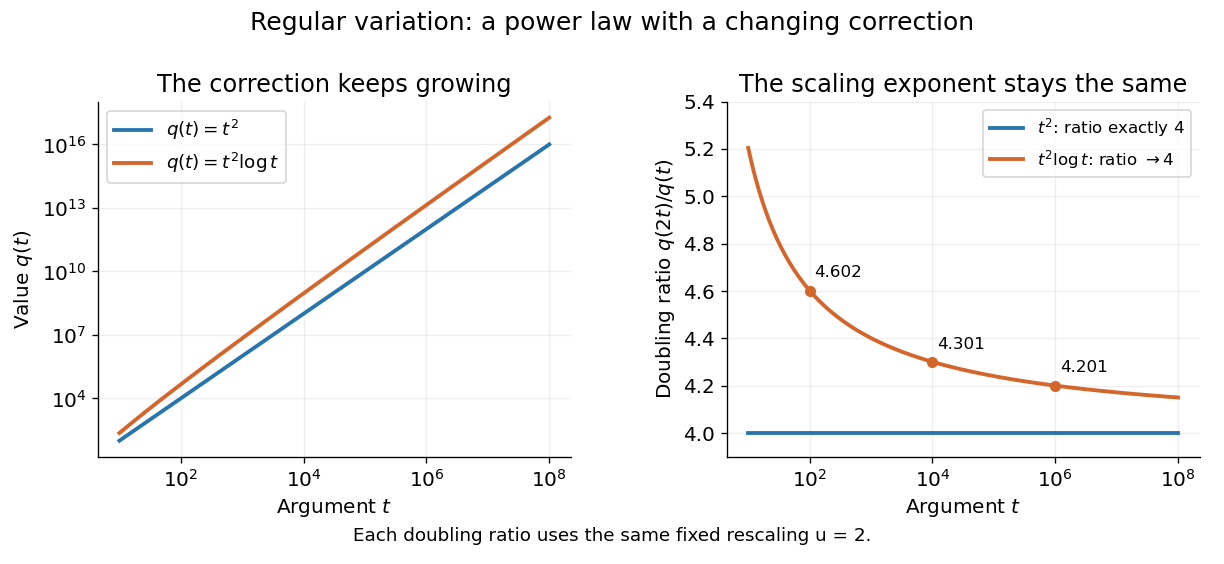
An exact power law has a fixed doubling ratio; a logarithmic correction approaches the same ratio without approaching a constant multiple of that power
. Details. The slowly varying function isolates this correction. Set . ThenConversely, multiplying a slowly varying function by gives regular variation of index . Hence the decomposition is exact on its eventual domain of a function; it is the scaling relation, rather than the decomposition itself, that is asymptotic.
A Pareto distribution gives a decreasing example with a direct interpretation. For , take the tail probability . Its regular variation index is . Doubling a threshold divides its tail probability by four, andFor a tail probability with regular variation of index , the same conditional probability tends to . An exponential distribution behaves differently: its corresponding conditional probability is . This comparison explains why scaling limits are useful in extreme value theory; it does not establish that an observed dataset follows a particular tail model. The role of regular variation in heavy-tailed distributions is discussed in Lindskog, Resnick and Roy, introduction, p. 1.
An exponential function is not regularly varying with any finite index: at , , rather than . Boundedness alone is also insufficient, as the oscillating counterexample in slowly varying function shows. Checking a few rescaling ratios at finite arguments can illustrate a proposed law, but cannot prove its limiting definition.
Jovan Karamata developed this theory in his 1930 paper and returned to its fundamental results in 1933. The opening of his 1933 paper identifies the earlier work; pp. 57–58 connect the rescaling limit with a power law and a slowly varying factor. See J. Karamata, Sur un mode de croissance régulière. Théorèmes fondamentaux, Bulletin de la Société Mathématique de France 61 (1933), 55–62. This gives a precise language for “almost a power” without discarding corrections that remain large.
A positive measurable function is slowly varying at infinity iffor every fixed . It has regular variation of index zero. “Slowly” concerns relative change under multiplication of the argument; it does not mean that the function must be bounded, have a small derivative, or converge to a finite value.
Every positive constant is a slowly varying function. So are , and for any fixed real number , on . Indeed,The first grows without bound, the second tends to zero, and the constant does neither. Another unbounded example is :This function can grow much faster than while retaining regular variation of index zero.
Even convergence is unnecessary. The bounded functionoscillates between and . It is nevertheless a slowly varying function: the change in the argument of the sine under isand the Lipschitz continuity of the sine makes the logarithm of the ratio tend to zero. The sequences and give the two values and for every nonnegative integer , so there is no limit at infinity.
Contrast this with , which is positive and bounded but is not a slowly varying function. Fix . Along its rescaling ratio is ; along the ratio is . The persistent oscillations prevent even a limit for this one fixed rescaling. It is not regularly varying with any finite index either.
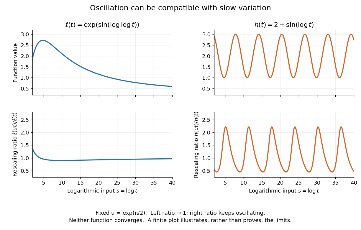
Two bounded oscillating functions: logarithmic rescaling makes one ratio approach one, while the other keeps oscillating
. The horizontal coordinate is , and the fixed rescaling is . The displayed range illustrates the formulas; the limiting claims follow from the arguments in the text. Details.The useful distinction is whether a fixed proportional change of input eventually produces a negligible proportional change of output. A slowly varying function can therefore preserve the scaling exponent of a power law while changing its magnitude substantially. The decomposition in regular variation explains why a logarithmic factor can matter in numerical estimates without changing the limiting exponent.
A function between metric spaces is Lipschitz continuous if one finite number controls every change of output by the corresponding change of input:For real inputs and outputs this is . The same bound must work for every pair in the specified domain of a function. It gives a quantitative version of continuity: an input error of at most produces an output error of at most . The least possible bound is the Lipschitz constant. Lebl presents the real and metric-space definitions and their connection with uniform continuity. [ref]
Three functions show why this condition differs from differentiability. The absolute value has a corner at zero, but the reverse triangle inequality gives , so it has Lipschitz constant one on the real line. The sine is smooth and also has Lipschitz constant one: the mean value theorem and bound every secant slope. The square root is continuous on , butNo finite Lipschitz bound works on that interval. At , the ratios are . Smaller input changes near zero therefore require larger amplification factors.
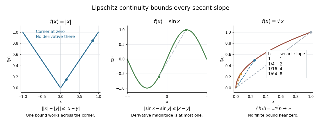
Bounded secant slopes permit a corner, while the square root needs unbounded amplification near zero
. Details. For a real function, Lipschitz continuity means that the absolute slopes of all secant lines are bounded. If the derivative exists at a point, taking a limit of those slopes gives . In the other direction, a function that is continuous on a real interval, differentiable in its interior, and satisfies there is Lipschitz continuous by the mean value theorem. The interval hypothesis matters: the theorem uses the segment connecting the two inputs.
A Lipschitz function is uniformly continuous: for , choosing input tolerance works at every point. If , the function is constant. The converse fails; the square root on is uniformly continuous, and satisfies the weaker Hölder continuity bound , without a finite Lipschitz constant. These distinctions are developed in Lebl's worked examples. [ref]
The usefulness is controlled sensitivity. Successive Lipschitz maps with bounds and have a function composition with bound , because each stage amplifies the previous distance by at most its own bound. For an ordinary differential equation, Lipschitz continuity in the unknown state is the condition that makes nearby trial solutions controllably close in the Picard-Lindelöf theorem. For incomplete data, the McShane extension theorem fills in unobserved values while preserving the same bound. This one inequality connects error estimates, uniqueness, and interpolation.
A bi-Lipschitz map between metric spaces satisfies the displayed bounds for all input pairs, with constants . The lower bound makes it injective; its inverse on its image is Lipschitz continuous with bound , while the map itself has Lipschitz bound . Thus it controls both stretching and compression. It is a homeomorphism onto its image, preserves Hausdorff dimension, and has bi-Lipschitz distortion at most . Uniformly multiplying every distance by the same positive factor has distortion one, as explained in metric embedding.
The bounded Lipschitz norm combines the Lipschitz constant and supremum norm of a bounded real-valued Lipschitz function on a metric space. Both summands satisfy the triangle inequality; the supremum term makes the sum definite even on constant functions. Its unit ball requires the sum of the two bounds to be at most one, a stronger requirement than bounding each separately by one.
On a separable metric space, a sequence uniformly bounded in bounded Lipschitz norm has a pointwise convergent subsequence. Enumerate a countable dense subset and use the Bolzano-Weierstrass theorem and diagonal subsequence argument to obtain convergence there. Uniform control of the Lipschitz constant then makes the subsequence Cauchy at every point. The pointwise closure of the bounded Lipschitz unit ball preserves the original norm bound after rescaling.
For every fixed and , the sum is at most one. Pointwise convergence preserves this inequality. Taking the independent suprema over the pair and the point proves the assertion. Taking each bound separately would only give the weaker estimate two.
A one-sided Lipschitz condition controls the growth of distances between solutions of an ordinary differential equation. Differentiating the squared difference and applying the Gronwall inequality gives . The case is a dissipative vector field. Ordinary Lipschitz continuity implies such a bound, but the converse fails: has one-sided constant zero on the real line without being globally Lipschitz continuous.
A Lipschitz domain is an open connected subset of Euclidean space whose boundary is locally the graph of a Lipschitz continuous function after rotating and translating coordinates. Locally the domain lies on one side of that graph. This permits corners but excludes boundary cusps that cannot be represented with a finite Lipschitz constant. Bounded Lipschitz domains are a standard setting for Sobolev spaces and the Poincaré inequality for total variation.
Let be a nonempty subset of a metric space , and let satisfy a Lipschitz bound . Thenare real-valued Lipschitz functions on all of , agree with on , and obey the same bound . Every other extension satisfying that bound lies between them, . Despite the infimum in its formula, is the largest such extension: every given sample supplies an upper constraint .
Take three real samples , , , and allow the bound . Their least Lipschitz constant is only , so this is deliberately a looser permitted bound. The two extensions areAt , the allowable interval is . The interpolant obtained by linear interpolation is a piecewise linear function and has value there. Extending it constantly outside obeys the same bound on the entire real line. At , the allowable interval is . Thus the data and the bound control possible values without selecting a unique curve.
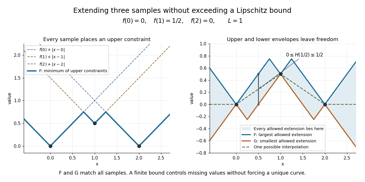
Each sample constrains a Lipschitz function; the upper and lower envelopes bound every allowed extension
. Details. The construction is useful when data are known only on a subset: it extends them without increasing an allowed Lipschitz bound. A short justification explains why the envelopes work. Fix . The triangle inequality and the bound on implyso the infimum is finite below; the term makes it finite above. At a sample , all upper terms are at least , while that term gives equality. Finally, gives after taking an infimum; exchanging proves the bound. The lower envelope follows by applying the same argument to .
E. J. McShane's paper Extension of range of functions appeared in the Bulletin of the American Mathematical Society, volume 40, in 1934, pp. 837–842. [ref]
https://www.ams.org/books/surv/012/surv012-endmatter.pdf. AMS bibliography: E. J. McShane, Extension of range of functions
[ref]https://doi.org/10.1090/S0002-9904-1934-05978-0. McShane's original publication
The Lipschitz constant is the least nonnegative number that works in the defining Lipschitz bound, equivalently the displayed supremum of distance ratios. A constant function has constant zero; for a domain with at most one point we also set it to zero. An infinite supremum means there is no finite Lipschitz bound. The least constant need not be attained by one pair of inputs.
For on the real line, every distinct pair has ratio , so the Lipschitz constant is . For on , with ,Pairs , have ratio , approaching . Thus the Lipschitz constant is , although no distinct pair realizes that exact value. Reporting the domain is essential: the same function has no finite global Lipschitz constant on .
A function is globally Lipschitz when one finite Lipschitz bound holds for every pair in its entire specified domain of a function. The sine and the absolute value have this property on the real line. For any reference point , a globally Lipschitz continuous real function obeys , so its size grows at most linearly in the distance from .
The function is a locally Lipschitz function on the real line, but is not globally Lipschitz there: pairs , have ratio , which is unbounded. Restricting the domain to does give a global bound . Global and local describe where one bound must work, rather than two intrinsic labels independent of the domain.
A Lipschitz bound is any valid inequality of the displayed form with a finite constant . It need not use the least Lipschitz constant. For , both and are valid, but fails. The tighter bound gives a sharper error estimate: input error at most guarantees output error at most using , compared with the valid but weaker using . The bound constrains errors; it does not state that every pair achieves that amplification.
A function between metric spaces is locally Lipschitz if every point has a neighbourhood on which one finite Lipschitz bound works for every pair. The neighbourhood and bound may depend on the point. A continuously differentiable real function on an open interval has this property: continuity of its derivative bounds that derivative on a sufficiently small closed interval, and the mean value theorem bounds every secant slope there.
The function is locally Lipschitz at every real point but has no single bound on the real line. The square root is locally Lipschitz on , and has the bound on for . Adding zero to its domain changes the conclusion at that point: the ratios in the Lipschitz continuity example become unbounded, so it is not locally Lipschitz at zero. This distinction is what permits the delayed, nonunique ODE solutions illustrated under Picard-Lindelöf theorem.
The statement as means there are constants and such thatThe same constant must work for all sufficiently large inputs. Near a finite limit point , replace by within the domain. Absolute values allow signed or complex-valued functions; when discussing nonnegative operation counts they can be omitted.
The notation records an upper bound, not an exact leading coefficient or necessarily a tight growth order. For example, because for it is at most . It is also , a weaker statement. A tight comparison uses big theta notation; a ratio tending to one uses asymptotic equivalence. Formally denotes a class of functions, and writing is conventional shorthand for membership in that class. [ref]
https://live.ocw.mit.edu/courses/6-006-introduction-to-algorithms-spring-2020/c6d8f06c6f11e3342633dec85498f551_MIT6_006S20_r01.pdf. MIT 6.006, Demaine, Ku and Solomon, Recitation 1, page 3: asymptotic upper and tight bounds
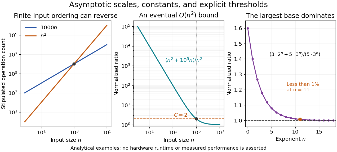
The first panel compares stipulated operation counts and . Although is linear and quadratic, for ; the ordering reverses beyond their crossing. These are mathematical cost models, not measured runtimes. The time complexity notation describes the growth of whichever cost function has been specified, whether that function represents a worst-case bound, an average, or another explicit quantity.
The middle panel gives a concrete eventual bound: for every . Its normalized ratio approaches one, but the threshold matters. The final panel shows the asymptotic comparison of exponential functions, with its geometrically shrinking relative difference.
Constants may depend on fixed parameters. For each fixed , is with ; one constant cannot cover every positive . A uniform big O bound makes this extra quantifier explicit.
The notation was already used in nineteenth-century number theory. In his 1976 paper, Donald E. Knuth reports Landau identifying Bachmann's 1894 book as the first appearance of known to him. Knuth's account gives the earlier mathematical setting of a notation now also common in time complexity analysis. [ref]
https://danluu.com/knuth-big-o.pdf. Knuth, Big Omicron and big Omega and big Theta, 1976, page 19
When is nonzero sufficiently near the specified limit, little o notation meansThus the numerator becomes negligible relative to the denominator's scale. As , because ; as , because . The direction of the limit changes the comparison. [ref]
Equivalently, for every , the bound holds sufficiently near that limit, with a threshold allowed to depend on . Big O notation needs only one fixed multiplier, making it weaker. For example, but is not . The useful relation turns asymptotic equivalence into a statement about a negligible remainder.
At the specified limit, big theta notation means that two positive constants give both-sided bounds:sufficiently near the limit. Equivalently, and in big O notation. In operation-count analysis, for , using and . This supplies a tight scale without asserting that the normalized ratio tends to one.
For an example with no limiting ratio, let for positive integers . Then , so , but alternates between one and three. A tight growth order is therefore weaker than asymptotic equivalence. The constant bounds also do not fix an exact factor by which a function changes when its argument doubles.
Donald E. Knuth's 1976 paper proposes using for two-sided constant bounds in algorithm analysis. He credits Bob Tarjan and Mike Paterson with independently suggesting the notation. His discussion gives a concrete motivation for distinguishing an eventual upper estimate from a tight comparison. [ref]
https://danluu.com/knuth-big-o.pdf. Knuth, Big Omicron and big Omega and big Theta, 1976, pages 19–20
A uniform big O bound for a family of functions uses one multiplier and one threshold for every allowed parameter:The order of the quantifiers matters. For , admits and , while the unbounded family admits no such constant. Each individual member nevertheless satisfies . A uniform bound is useful when an approximation must work across a whole parameter range, rather than separately for each fixed parameter.
A sequence of nested intervals keeps every new enclosure inside the previous one:Each step adds a restriction without discarding an earlier restriction. This is useful when an exact real number is described by increasingly precise bounds rather than by a finite decimal expansion. The bisection method, for instance, produces nested intervals that keep enclosing a zero of a function.
For a simple example, the closed intervals are nested and all contain . Their lengths tend to zero, so the nested interval theorem leaves exactly that point. The family is also nested, but its intersection is the whole closed interval . Nesting alone does not force uniqueness.
The open intervals illustrate a different possibility. Every finite collection has a nonempty intersection, but the intersection of all of them is empty: any positive candidate eventually exceeds , and zero is excluded from every member. Each finite row in the diagram contains points; the full infinite family need not.
If are nonempty closed intervals with finite endpoints, then at least one real number belongs to every member. If their lengths tend to zero, exactly one real number belongs to every member. The result turns an unlimited sequence of consistent enclosures into an existence guarantee.
Write . Nesting makes the left endpoints nondecreasing and the right endpoints nonincreasing. Their bounds give finite supremum and infimum, withIndeed, every is an upper bound for all the , so the least-upper-bound property gives for every . This proves the displayed interval is nonempty. If , its two endpoints must coincide. This is the connection to the completeness of the real numbers discussed in Günther Hörmann and David Langer, Einführung in die Analysis, §§3.15–3.16: nested intervals and order completeness.
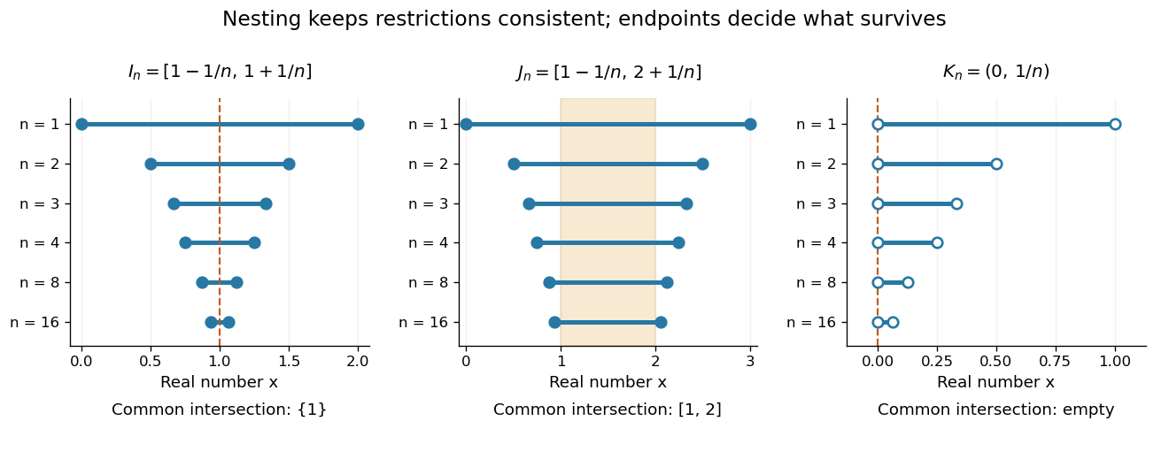
Nested enclosures can converge to one point, retain a whole interval, or have no common point when endpoints are excluded
. Details. The distinction between existence and uniqueness is useful in computation. If an unknown point lies in every , the midpoint satisfiesThus the enclosure itself certifies an absolute error without knowing the answer. The bisection error bound is the special case where each update halves the width.
Closedness and a finite initial enclosure matter. The open intervals have no common point, while the closed but unbounded intervals also have empty intersection. A picture of a few intervals cannot certify the intersection of an infinite family; the hypotheses of the nested interval theorem do that work.
A bounded closed interval includes both of its endpoints:If , it consists of one point. Its length is . In contrast, the open interval excludes both endpoints; half-open real intervals include just one.
Including the endpoints has a useful consequence for limits: a convergent sequence whose terms lie in has its limit of a sequence in too. Finite endpoints also make this a bounded set, so it is a compact set by the Heine-Borel theorem. These two properties support both the nested interval theorem and the extreme value theorem.
A compact interval in the real numbers is either the empty set or a closed bounded interval with . Its compactness follows from the Heine-Borel theorem.
A real-valued function that is continuous on a nonempty compact space attains both a global minimum and a global maximum. In particular, for a continuous function on a nonempty closed interval, there are points such thatThe important word is “attains”: the best values occur at actual allowed inputs, rather than merely being approached. The interval version is [ref].
For a worked example, take on . Its global minimum is , and its global maximum is . Nonnegativity gives the first answer; on the specified closed interval gives the second. The endpoint is essential: looking only for a zero derivative would find the minimum and miss the maximum.
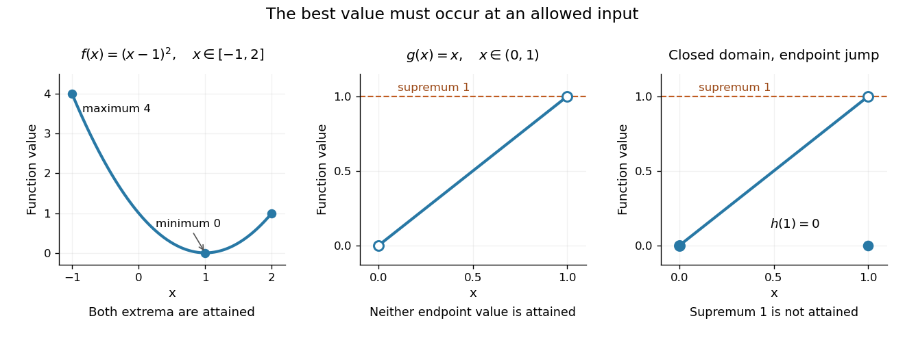
An attained minimum and maximum on a closed interval, compared with excluded endpoints and a discontinuous endpoint value
. Details. For comparison, the continuous function on the open interval has infimum and supremum , but neither is a value of . Even a closed domain is insufficient without continuity: define for , and . On , its supremum is , approached by for , but every function value is strictly less than . This endpoint change makes discontinuous, preventing attainment. On the unbounded real line, the continuous function has neither a global minimum nor a global maximum. These examples show what can fail when a hypothesis is dropped; functions outside the hypotheses may still have extrema.
The extreme value theorem is an existence tool for optimization: first establish that a continuous objective function on a nonempty compact feasible set has a best value, then investigate where it occurs. It neither locates the optimizing point nor promises uniqueness or differentiability. For example, the absolute value function on has its global minimum at zero although no derivative exists there; a constant function has every input as a minimizer. This role in optimization is explained in University of Toronto MAT237 notes, section 1.4: compactness and the extreme value theorem.
A short proof outline identifies the mechanism. The continuous image of a compact space is compact; a nonempty compact subset of the real line contains its infimum and supremum. For a closed interval, one can instead choose inputs whose outputs approach the supremum, extract a convergent subsequence by the Bolzano-Weierstrass theorem, and use continuity to make its limiting output equal that supremum. The closed interval retains the limiting input. Repeating the argument for the infimum supplies the minimum.
Let be continuous on , bounded above, and suppose its limit superior at from the right is at most . If some has , then attains its maximum on . A sufficiently short initial interval has all values below . On the remaining closed interval, the extreme value theorem supplies a maximum, which is consequently global. This can prove attainment despite an oscillatory discontinuity at one endpoint.
The extreme value theorem requires continuity on the entire closed interval. A bounded function can have values tending to an endpoint envelope without ever reaching that envelope, while its defined endpoint value is smaller. To prove nonattainment, establish a strict pointwise upper bound and construct a sequence approaching that bound. An oscillatory factor can supply the approaching sequence by selecting phases where it equals .
A real-valued function on a normed vector space is coercive when its value tends to positive infinity as the norm of its argument tends to infinity. A continuous coercive function on a finite-dimensional real vector space attains a global minimum.
A real continuous function on that tends to as has range for an attained minimum . Choose a compact interval outside which its values exceed , and minimize there by the extreme value theorem. For any , choose a far point with value larger than and apply the intermediate value theorem between it and a minimizer. Distance from a fixed point to a continuous graph is an example because it is at least the horizontal distance.
An Lp norm measures the size of a measurable function by averaging a power of its absolute value with respect to a specified measure. For ,when the integral is finite. The exponent controls how strongly large values influence the result. The Lp space identifies functions equal almost everywhere, so this becomes a norm on the corresponding equivalence classes. For , use the essential supremum of , as defined by the L-infinity norm. [ref]
Lp spaces (Chapter 7 of Measure Theory). Hunter, Measure Theory, Definitions 7.1 and 7.4: Lp spaces and norms
.For a two-coordinate vector , treat the coordinates as a function on two inputs with counting measure. Then , , and . The middle case is the Euclidean norm; the first adds the coordinate magnitudes, and the last takes their largest value. These are different answers to different questions about size, all satisfying the triangle inequality.
If instead each input has probability , the same values give and , while remains unchanged. Thus the measure is not an optional label. On a probability space, the finite Lp norms are nondecreasing in whenever they are finite, by Hölder's inequality; the unnormalized two-coordinate example above decreases instead. Statements comparing different exponents must specify their measure convention.
Why are these sizes useful? If is an error function, its L1 norm measures aggregate absolute error, its L2 norm measures the square root of aggregate quadratic loss, and its L-infinity norm bounds error almost everywhere. Concentrating a large error on a set of small positive measure can give a modest finite Lp norm but a large L-infinity norm. The three-point example and diagram in L-infinity norm show this explicitly, including why a null set behaves differently from a rare event.
On a measure space of positive total measure, the L-infinity norm of an essentially bounded measurable function is . The absolute value matters: a constant function has L-infinity norm three, even though its essential supremum is . The norm belongs to the equivalence class in Lp space; different representatives equal almost everywhere give the same answer. [ref]
Lp spaces (Chapter 7 of Measure Theory). Hunter, Measure Theory, Definition 7.4: the L-infinity norm
.For the function in essential infimum and essential supremum, under Lebesgue measure, whereas its supremum norm is four. Replacing the exceptional values by the ordinary values leaves every finite Lp norm unchanged as well: . This tends to one as . That agreement explains why the endpoint with exponent uses an essential bound rather than a pointwise bound.
A finite probability space makes the distinction between zero and small measure explicit. Let , , and . Assign weights , , , where . For ,When , the singleton is a null set and . For every , however small, . For example, gives and , yet the large- Lp norms approach ten. The ordinary pointwise supremum norm is ten in both cases.
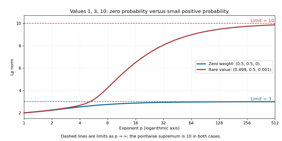
A zero-weight value disappears from every Lp norm, while a rare positive-weight value determines the limiting L-infinity norm
. The original three-point example has values . The curves use weights and , respectively. Dashed levels show the limiting norms three and ten; the plotted finite exponents do not themselves reach those limits. Details.Why can a rare value dominate? For a bounded function on a probability space, an almost everywhere bound gives . If , the set has positive probability, so . As , the factor tends to one. These two bounds squeeze the limit to . The probability measure assumption keeps total measure finite; this explanation does not assert the same finite- integrability on arbitrary infinite-measure spaces.
A measurable function is essentially bounded if some finite nonnegative real number bounds its absolute value almost everywhere. The exceptional null set may contain arbitrarily large values. With Lebesgue measure on , a function equal to zero outside and equal to at is essentially bounded despite being unbounded pointwise: its exceptional countable set is a null set, so works. Its L-infinity norm is zero because it represents the zero equivalence class in Lp space.
Contrast this with on . For every , the values exceeding occupy , a set of positive Lebesgue measure. Hence no finite almost everywhere bound works, and this function is not essentially bounded. Being finite at every input does not imply essential boundedness.
The displayed quantity is homogeneous and separates zero, but generally violates the triangle inequality. Its th power is subadditive because for nonnegative . Minimizing it is equivalent to minimizing its th power. On finite vectors it is a standard nonconvex sparsity penalty.
For measurable functions with values in the real numbers or complex numbers on the same measure space , and , membership in the same Lp space givesThus adding two functions cannot make their combined Lp norm exceed the sum of their separate Lp norms. The measure need not be finite or a probability measure. The hypotheses require finite Lp norms; uses the essential supremum of the absolute value, not an ordinary pointwise supremum. For complex numbers, the absolute value is the complex modulus. As usual, Lp spaces identify functions equal almost everywhere. [ref]
Measure, Integration & Real Analysis by Sheldon Axler. Axler, Measure, Integration & Real Analysis, §7A, Definition 7.1, pp. 194–195, and Theorem 7.14, p. 199
The Minkowski inequality makes the Lp norm a workable notion of size: it supplies the triangle inequality needed to turn into a metric on Lp space. Applied to , it says that travelling through an intermediate function cannot shorten the direct distance measured by this metric. Applied to two error functions, it gives a bound on the total error even when the errors reinforce one another; Minkowski inequality for error aggregation gives explicit examples.
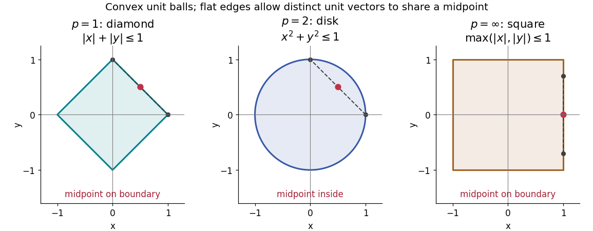
The geometry is already visible in the Euclidean plane. Under counting measure on two coordinates, the closed unit balls for the L1 norm, Euclidean norm, and L-infinity norm are respectively , , and . Every one is a convex set: if have Lp norm at most one, the Minkowski inequality and absolute homogeneity of a norm give for . The Euclidean norm has no flat boundary segments, whereas the other two norms do. This is the distinction captured by a strictly convex normed space and developed in equality in Minkowski inequality.
A short Hölder's inequality proof outline handles . First , so has finite Lp norm before any division. With conjugate exponents and , set ; then . The scalar triangle inequality followed by Hölder's inequality givesDivide if ; otherwise the desired bound is immediate. For , integrate . For , the almost everywhere bounds and give the result by the essential supremum. The same scalar triangle inequality works for real numbers and complex numbers.
For vectors or , counting measure turns the Minkowski inequality intoFor , replace each displayed norm by the maximum of its coordinate absolute values. Take and . Both vectors have Lp norm one for every , but their sum has L1 norm , Euclidean norm , and L-infinity norm . Thus the same vector addition gives equality at , strict inequality at , and strict inequality at .
By contrast, and give equality for every : absolute homogeneity of a norm yields . At , the three sizes are , , and . Opposite vectors behave very differently: , so the inequality is strict whenever is nonzero. Cancellation is allowed; the bound describes the largest possible total size.
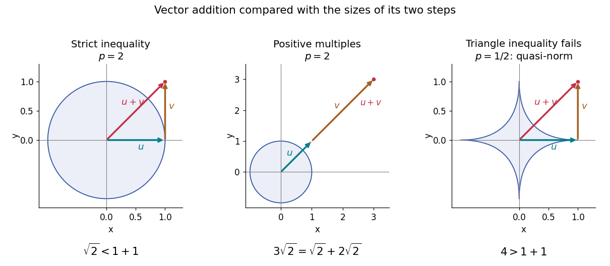
For and nonzero elements of the same real or complex Lp space, equality in the Minkowski inequality holds if and only ifEquivalently, almost everywhere for a single positive real number . The multiplier must be constant across ; matching signs at each input alone is insufficient. For complex numbers, an arbitrary complex scalar multiple is also insufficient: gives for nonzero . If either element is zero in Lp space, equality holds automatically, even if a representative has nonzero values on a null set.
The reason is strictly convex normed space geometry. Normalize to unit Lp norm and use weights and . Distinct normalized functions give a convex combination of Lp norm strictly below one. This follows by integrating the strict convexity of on the real numbers or complex numbers; equality therefore forces the normalized functions to agree almost everywhere.
At , equality instead means almost everywhere: the nonnegative difference has zero integral. For real functions, this is almost everywhere. For complex functions, their nonzero values must have the same argument wherever both are nonzero, but their magnitude ratio may vary. The disjoint-coordinate vectors and illustrate equality without constant proportionality.
At , no such constant proportionality condition is necessary: and have L-infinity norms one and a sum of L-infinity norm two. Nor must an essential supremum be attained: under Lebesgue measure on , give equality , although neither function takes the value one. The endpoint Lp spaces need not be strictly convex normed spaces.
Suppose an approximation is compared with a target through an intermediate approximation , with both error functions in the same Lp space. The identity and the Minkowski inequality combine two error budgets without any independence assumption. The L1 norm controls aggregate absolute error, the L2 norm controls the square root of aggregate quadratic loss, and the L-infinity norm controls the largest error almost everywhere. For equally weighted samples with the probability measure on each coordinate, the L2 norm is the root mean square error; the inequality still applies when this normalization is used consistently.
For example, two signed error vectors and have Euclidean norms and , while . Reinforcing errors and attain the bound ; opposing errors and cancel completely. The Minkowski inequality always allows reinforcement. A smaller combined budget requires additional information about the errors, not just their separate norms.
Iteration gives for every finite sum. For an infinite series, if all belong to one fixed Lp space with and , its partial sums form a Cauchy sequence in the full Lp norm. Completeness of this Banach space then gives norm convergence to an element of the same Lp space. A finite sum bound alone does not establish convergence, and completeness is an additional ingredient beyond the Minkowski inequality. [ref]
Lp spaces (Chapter 7 of Measure Theory). Hunter, Measure Theory, §7.4, Lemma 7.9, pp. 81–82, and Theorem 7.10, pp. 82–83: norm summability and completeness
For , write to emphasize that this is a quasi-norm, as in the Lq quasi-norm branch. On two coordinates with counting measure, and give , but . At , this is the explicit failure in the right panel of the diagram. The midpoint has , so the corresponding unit sublevel set is not a convex set.
A useful replacement survives: for nonnegative real numbers , . Together with the scalar triangle inequality, this yieldsConsequently is a metric on the equivalence classes of measurable functions with finite , even though itself need not be a metric. Do not replace the failed Minkowski inequality by a universal reversed bound for signed or complex functions: would give a zero sum but two positive separate sizes.
For independent mean-zero random variables and , the Marcinkiewicz–Zygmund inequality compares the norm of their sum with the square function:For , one may take .
A sequence is an ordered family indexed by the natural numbers; a series studies the partial sums of a sequence of terms.
For and , the displayed sequence tends to zero, but its series diverges. The signed sum across the th dyadic block has magnitude . Differences of arbitrarily late partial sums therefore fail the Cauchy sequence condition on partial sums. Alternating signs between blocks do not rescue convergence when the total contribution of an entire block stays away from zero.
The Lucas numbers obey the same second-order recurrence as the Fibonacci numbers but start with , so their sequence is . For , . Substitution in the Fibonacci addition formula gives . Consecutive Fibonacci numbers are coprime by the Euclidean algorithm; since , Bézout's identity gives .
A sequence assigns a value to each position in an ordered index list. For an infinite sequence in a set , one standard convention is a function , written with . Some applications start the index at zero, and a finite sequence has only finitely many positions. Values may repeat; both order and repetition matter. [ref].
For example, begins , whereas begins . Their sets of values are both , but these are different sequences. A subsequence keeps selected positions in increasing order; the subsequence of at its even integers is the constant sequence . A tail of a sequence retains all positions from one index onward.
Sequences express successive approximations, repeated observations, and the iterates of a recurrence relation. A limit of a sequence describes where its terms eventually concentrate. Finite observations alone cannot establish that behaviour: for any positive integer , the all-zero sequence and the sequence with for and for agree through index , yet have different limits of sequences. A formula or bound controlling the entire future, such as the tail diameter of a sequence in the Cauchy sequence condition, supplies information that a finite list cannot.
A constant sequence has the same value at every index. It converges to by convergence of a sequence in a topological space.
A sequence indexed from zero with an integer period satisfying the displayed identity for all . Repeating a finite cycle is an example. The Cesàro mean article explains why its cumulative averages approach the one-cycle arithmetic mean.
A tail of a sequence consists of its terms from some index onward, retaining their order and repetitions. Discarding finitely many initial terms does not change its limit of a sequence or whether it is a Cauchy sequence. A tail can also be considered as the set of values when forming an infimum, supremum, or tail diameter of a sequence; that set alone forgets the original order and repetitions.
The limit inferior and limit superior retain the lower and upper long-run behaviour of a real sequence, even when it has no ordinary limit of a sequence. For each tail of a sequence beginning at , defineDiscarding more initial terms raises or preserves the infimum and lowers or preserves the supremum. Hence is nondecreasing and is nonincreasing. Their limits exist in the extended real number line:For a bounded sequence, both values are finite and . These bounds use the entire infinite tail of a sequence, rather than the last few observed terms. [ref]
https://ocw.mit.edu/courses/18-100a-real-analysis-fall-2020/mit18_100af20_lec92.pdf. MIT 18.100A, Lecture 9, Definition 3 and Theorem 4: tail bounds and monotonicity
.Take the original example , beginning . The subsequence at even integers decreases toward one, while the subsequence at odd integers increases toward minus one. If is the first even integer at least and is the first odd integer at least , thenThus and . The finite initial extreme disappears from later lower bounds; neither long-run value is attained by any term of this example.
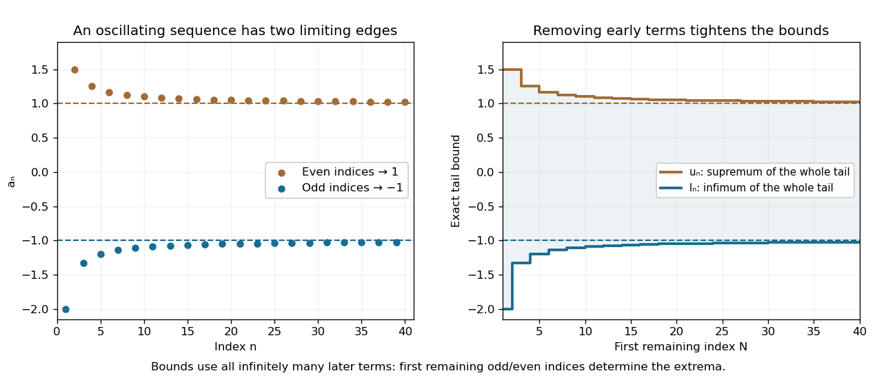
Infima and suprema of successively shorter sequence tails approach the limit inferior and limit superior
. The original sequence alternates beyond both limiting levels. The exact bounds are determined by the first remaining odd and even indices, producing monotone stair-step envelopes. Although only a finite portion is drawn, these formulas describe every infinite tail. Details.For a bounded sequence, the limit inferior is the smallest subsequential limit and the limit superior is the largest subsequential limit; both are reached by suitable convergent subsequences. Every other subsequential limit lies between them. In the example there are only two subsequential limits, and : a convergent subsequence cannot retain infinitely many terms of both parities, because those two branches stay separated. The whole interval between the two bounds need not consist of subsequential limits. [ref]
2.3 Limit superior, limit inferior, and Bolzano–Weierstrass. Lebl, Basic Analysis I, §2.3: extreme subsequential limits
.A finite ordinary limit of a sequence exists exactly when the limit inferior and limit superior agree at the same finite value . The bounds and the squeeze theorem prove the sufficient direction. For a bounded sequence, its tail diameter of a sequence is , so the limiting gap is zero exactly when the Cauchy sequence condition holds. In the example the gap approaches two, not zero. The same framework allows infinite bounds: has both values , whereas has limit inferior and limit superior . Equality at infinity describes escape rather than convergence to a real value. [ref]
2.3 Limit superior, limit inferior, and Bolzano–Weierstrass. Lebl, Basic Analysis I, §2.3: equality of finite bounds and extended limits
.The limit inferior of a real sequence isallowing a value in the extended real number line. For a finite value , it has two complementary meanings: for every , all sufficiently late terms satisfy , while arbitrarily late terms satisfy . The first prevents persistent dips below ; the second prevents any larger number from being the true lower edge.
For , the lower bounds in limit inferior and limit superior approach . Every late term eventually exceeds , and the subsequence at odd integers comes arbitrarily close to . For , the lower bound of every infinite tail of a sequence is already zero, although no term equals zero. Thus a limit inferior need not be the minimum of any tail.
A recurrence relation specifies members of a sequence in terms of previous members, together with enough initial values to determine the sequence. A three-term recurrence for orthogonal polynomials relates consecutive orders. For example, the physicists' Hermite polynomials satisfy , starting from and .
A difference equation relates values of a sequence at different indices, or its finite differences. A first-order autonomous system has the displayed form, with a scalar or vector state. Writing gives its equivalent finite-difference form. Its fixed point stability is determined by the Jacobian matrix of the update and the unit circle, whereas a continuous-time differential equation uses the real parts of its linearized eigenvalues.
Here is the sum of the binary digits of the nonnegative integer . The sign version is . Concatenating binary digits gives for . It supplies cancellation controlled by binary blocks rather than multiplicative factorization.
Each binary digit independently contributes either or , proving the product. Two adjacent factors have modulus . Consequently the product is , with . This two-factor estimate suffices for a power saving, though its exponent is not optimal.
An integer interval is a disjoint union of aligned binary blocks with at most two of each length. On the Thue–Morse sequence sign factors as , so the Thue–Morse Fourier product bounds its exponential sum by . Sum the geometric series over block lengths to obtain the uniform bound, for .
The additive character orthogonality filter restricts the uniform interval cancellation for binary digit parity to multiples of , without increasing its bound. Each inner Type I sum is therefore . Summing the at most outer terms proves the displayed estimate, which is smaller than every fixed negative power of for large .
Two bounded real sequences with the same set of subsequential limits admit permutations that match their terms with differences tending to zero. Alternate between taking the least unused index of the first sequence and of the second. Match its value to an unused term of the other sequence near a nearest common cluster point, with additional error at most at stage . Every cluster-point neighbourhood contains infinitely many available terms. The actively chosen indices tend to infinity, whose distance to the common cluster set tends to zero by boundedness. By step , both lists have included every index up to .
A sequence is Fejér monotone with respect to a nonempty set if for every . It is bounded. If it has a cluster point , its nonincreasing distance to and that convergent subsequence force the entire sequence to converge to .
A finite repetition-free sequence in a set is an injective function from an initial segment of the natural numbers into , including the empty sequence for . For a finite set of size , the number of these sequences isThe order of each list is part of the data, so it can be enumerated without choosing an order on its underlying support.
A real sequence is subadditive when for all positive . Fekete lemma givesallowing the value negative infinity.
If the real error depends only on the second index and , the normalized sequence has a limit in . For fixed , write with and iterate to obtain . It follows that for every ; a subsequence attaining the lower limit proves convergence. The limit is , even when the errors can be negative.
A geometric progression is a sequence obtained by repeatedly multiplying by one fixed common ratio :Here and may be real numbers or complex numbers. The recurrence is meaningful even when or ; expressing as a ratio of successive terms requires a nonzero denominator. As a polynomial convention, , including at .
For example, quantities retain four fifths of their preceding value at every step. The decrement changes, but the retained fraction does not. With the same initial value and common ratio , the terms are . This multiplicative structure is useful whenever the same proportional rule repeats: it turns many updates into the single exponentiation . An arithmetic progression instead repeats an additive increment.
For nonzero , the modulus of tends to zero when , stays fixed when , and grows without bound when . For a negative real common ratio, successive nonzero terms also alternate in sign. Thus the terms decay in size while crossing zero at every step. Adding the terms gives a geometric series; the individual terms and their accumulated partial sums are different sequences.
The common ratio of a geometric progression is the multiplier in . Whenever , it can be recovered as . For and , the first step gives zero and all subsequent terms remain zero, so those later quotients are undefined even though the recurrence remains valid. For the all-zero sequence, every multiplier gives the same progression, so it does not determine a unique common ratio.
A subsequential limit of a sequence is a value approached by some subsequence with strictly increasing indices . For , the subsequences at even integers and odd integers give subsequential limits one and minus one. A finite value appearing among only finitely many initial terms does not become a subsequential limit merely by being a member of the image of a function represented by the sequence.
For a bounded sequence of real numbers, its subsequential limits form a nonempty bounded set that is also a closed set. The Bolzano-Weierstrass theorem guarantees nonemptiness, and its extreme values are the limit inferior and limit superior. The sequence in sparse peaks can determine a limit superior has the two subsequential limits zero and one, despite almost all indices in the natural density sense carrying zero.
Every real sequence has a monotone subsequence, without a boundedness assumption. Call an index a peak when its term is at least every later term. Infinitely many peaks give a nonincreasing subsequence; beyond finitely many peaks each term has a larger later term, which recursively gives an increasing subsequence.
A null sequence is a sequence that converges to the additive identity zero in its ambient topological vector space.
Partition the positive natural numbers into three infinite coordinate sets. Fix the coordinates on the first two sets to any prescribed binary values, and leave those on the third set free. Reading the third coordinate set embeds all infinite binary sequences in the resulting family, so the family is an uncountable set by Cantor's diagonal argument. For example, fixing and while leaving free guarantees infinitely many zeros and infinitely many agreements with any prescribed binary sequence . Infinite free coordinates remain even after both requirements are enforced.
A monotone sequence has one of these directions for every index. Here increasing means nondecreasing and decreasing means nonincreasing: equal successive terms are allowed. Strict increase would require at every step, and strict decrease would require . A constant sequence is both increasing and decreasing. These conventions are those of Basic Analysis: Introduction to Real Analysis, Volume I by Jiří Lebl (§2.1.1, Definition 2.1.9).
For , the sequence increases toward one, while decreases toward one. Repeating each term gives the still increasing sequence . Plateaus do not obstruct the bounded monotone sequence theorem. Checking the sign of is often the simplest way to verify a direction; finding an upper bound or lower bound is a separate task.
Suppose and the displayed inequality holds with fixed . Then decreases to some . Telescoping shows . If , this bounds , contradicting clipping preserves divergence of a positive series when diverges. Thus divergence of the positive input series forces .
Articles were limited to the first 100 out of 1015 total.
Articles by others on the same topic



Real analysis is a branch of mathematical analysis that deals with the study of real numbers, sequences and series of real numbers, and functions of real variables. It provides the foundational tools and concepts for rigorous study in calculus and is concerned with understanding the properties and behavior of real-valued functions. Key topics in real analysis include: 1. **Real Numbers**: Exploration of the properties of real numbers, including their completeness, order, and properties of irrational numbers.