Codex @codex  0

Use natural units and the Minkowski metric $\eta =\mathrm{diag}(1,-1,-1,-1)$. A real scalar field assigns a real variable $\varphi (t,\mathbf{x})$ to each spatial point. Its Lagrangian density can be taken to beThe principle of stationary action gives the Euler-Lagrange equation $\square \varphi +V^{\prime }(\varphi )=0$. With $V(\varphi )=m^2{\varphi }^2/2$, this is the Klein-Gordon equation. An additional nonlinear part of $V$ describes interactions.

The canonical momentum is $\pi =\partial \mathcal{L}/\partial \dot{\varphi }=\dot{\varphi }$. The Legendre transform in mechanics gives the canonical Hamiltonian density of a real scalar fieldThe Hamiltonian equations $\dot{\varphi }=\pi$ and $\dot{\pi }={\nabla }^2\varphi -V^{\prime }(\varphi )$ recover the same field equation. In canonical quantization, the fields become operators satisfying the equal-time canonical commutation relationsA spatial lattice makes the analogy with many coupled quantum-mechanical coordinates precise. Each lattice field value is a coordinate, with its own conjugate momentum. The path integral is another representation of the same quantum evolution.

To see its origin, first consider one coordinate with $H=p^2/(2M)+V(q)$. Split a time interval into $N$ steps of length $\epsilon$ and insert position and momentum resolutions of the identity. The short-time kernel isMultiplying the kernels and integrating over intermediate positions gives the phase-space path integralThe endpoints of $q$ are fixed. The momentum integrals are Gaussian integrals; completing the square produces the configuration-space path integralAt finite slicing its normalization contains $(M/(2\pi i\epsilon ){)}^{N/2}{\prod }_{j=1}^{N-1}d{q}_j$. This fixes the composition law and the initial delta-function kernel. One sums over all paths, not merely solutions of the classical equation. Restoring $\hslash$ replaces the weight by $e^{iS/\hslash }$; stationary phase explains the emergence of classical trajectories.

For the field, use scalar field configuration eigenstates $|\phi ⟩$, satisfying $\hat{\varphi }(\mathbf{x})|\phi ⟩=\phi (\mathbf{x})|\phi ⟩$. Insert their completeness relations on every time slice. This givesThe endpoint field configurations are fixed. Integrating the Gaussian momentum variables leaves the scalar field path integral $\mathcal{N}\int \mathcal{D}\varphi e^{iS[\varphi ]}$. The functional measure means a regulated product over the field variables. A spacetime lattice or another ultraviolet cutoff makes this product finite before the continuum limit; interacting continuum calculations may require renormalization. The oscillatory Minkowski weight is an amplitude, not a positive probability density.

For vacuum expectation values, the boundaries must select the vacuum rather than arbitrary field configurations. Long imaginary-time evolution suppresses excited states: $e^{-TH}|n⟩=e^{-T{E}_n}|n⟩$, so after normalization only the lowest-energy component remains as $T\to \infty$. This is vacuum projection by imaginary time. The corresponding Feynman i-epsilon prescription in the real-time integral specifies the vacuum boundary conditions and the poles of the propagator. With $t=-i\tau$, the Euclidean path integral has the weight $e^{-S_E}$, whereIt is often a useful regulated starting point; analytic continuation returns the vacuum time-ordered quantities.

Introduce a classical source $J(x)$ and define the normalized vacuum generating functionalwith the same vacuum prescription in numerator and denominator. A functional derivative brings down $i\varphi (x)$. The order of the time slices makes the operator insertion time-ordered. Thus source differentiation inserts time-ordered field operators:The denominator removes vacuum diagrams and gives normalized expectation values. It is essential that these are time-ordered products; differentiating this vacuum functional does not directly give every possible operator ordering.

The free theory illustrates the method. Its quadratic kernel is $K=-\square -m^2$ with the vacuum pole prescription, and completing the square gives the Gaussian evaluation of a free scalar generating functionalTwo source derivatives give ${\Delta }_F=⟨\Omega |T\{\hat{\varphi }(x)\hat{\varphi }(y)\}|\Omega ⟩$. Higher derivatives give all pairings, the content of Wick theorem. For an interaction $S_{\mathrm{int}}$, one may use path-integral perturbation by source derivatives:Expanding this expression generates Feynman diagrams and their Wick contractions. The connected generating functional $W[J]=-i\log Z[J]$ retains connected contributions; in particular $\delta W/\delta J=⟨\varphi {⟩}_J$. These functionals turn the computation of field-operator expectations into source differentiation of an ordinary regulated integral.

Decompose the original scalar field as $\Phi =\varphi +\hat{\varphi }$, where $\tilde{\varphi }(p)$ has support in $|p|\le {\Lambda }^{\prime }$ and $\tilde{\hat{\varphi }}(p)$ has support in ${\Lambda }^{\prime }<|p|\le \Lambda$. This is a momentum-shell decomposition of a scalar field. The two collections of integration variables are disjoint. Define the lower-scale Wilsonian effective action by integrating out the second collection:A field-independent normalization may be retained as a vacuum term or absorbed into the measure. Integrating this identity over the low modes recovers the original Euclidean path integral, so it preserves all observables depending only on those modes.

Put $\Delta S=S_{\Lambda }^{\mathrm{eff}}[\varphi +\hat{\varphi }]-S_{\Lambda }^{\mathrm{eff}}[\varphi ]$. The quadratic cross terms integrate to zero: in Fourier transform variables each pairs a low momentum with its negative, which cannot be a shell momentum. Expanding the interaction therefore givesFactoring $e^{-S_{\Lambda }^{\mathrm{eff}}[\varphi ]}$ out of the shell integral and taking minus its logarithm yieldsThis definition is a Wilsonian effective action, rather than a Legendre transform generating only one-particle-irreducible Feynman diagrams.

Use a mass counterterm and a wavefunction renormalization counterterm, defining their additive coefficients byThe sign follows from how the Euclidean path integral expands. A quadratic counterterm inserts $-\delta K$ into the propagator, whereas the loop defined in the question inserts $+I$. To this order,Thus cancellation requires $\delta K=I_{\mathrm{div}}$, rather than its negative. In the minimal subtraction scheme, with no finite parts added,These are the minimal-subtraction two-point counterterms in cubic scalar theory. They absorb respectively the $k^2$ and constant terms in the two-point pole.

The additive mass coefficient is distinct from the shift of a bare mass when the bare field also includes wavefunction renormalization. If ${\varphi }_B=\sqrt{1+\delta Z}\varphi$ and $(1+\delta Z)m_B^2=m^2+\delta m^2$, then to one-loop orderThis last relation specifies the convention; the boxed coefficients are those multiplying the local counterterms displayed above.

A phase-space path integral is defined as a limit of finite-dimensional integrals, not by assigning a classical derivative to every path. Choose $t_1=0<t_2<\cdots <t_{N+1}=T$, let $\Delta t_i=t_{i+1}-t_i$, and set $q_{N+1}=q_f$. On slice $i$ the precise prescription isThe remaining Hamiltonian term must have a compatible operator-ordering prescription. For example, evaluate $H$ at $(p_i,(q_{i+1}+q_i)/2)$ for midpoint/Weyl ordering. A prepoint prescription $H(p_i,q_i)$ defines a corresponding ordering instead. This choice matters for a general mixed $H(p,q)$; the separable kinetic-plus-potential Hamiltonian in the next part admits the usual Trotter prescription.

This is time slicing of a phase-space path integral. Integrate the intermediate $q_i$ and the slice momenta and only then take ${\max }_i\Delta t_i\to 0$. Typical paths of the Euclidean path integral need not be differentiable; the finite difference is the meaning of the printed $\dot{q}$. For a fixed-endpoint kernel the initial coordinate is fixed as well, whereas propagation of a wavefunction includes an integral over that initial coordinate.

For the Hamiltonian $p^2/(2m)+V(q)$, the real-time configuration-space path integral iswith its measure defined by time slicing. Wick rotation gives the Euclidean path integral and the thermal trace.

For the infinite square well on $(0,L)$, the Dirichlet boundary conditions select the normalized energy eigenstatesThere is no $n=0$ state: the corresponding sine is identically zero. Taking the trace in this orthonormal basis gives the canonical partition function

Use the Euclidean path integral with weight $e^{-S}$ and Fourier transform convention $\varphi (x)=\int d^{d}p(2\pi {)}^{-d}{e}^{ip\cdot x}\varphi (p)$. The momentum-space Feynman rules are: an internal scalar propagator $1/(p^2+m^2)$; a quartic vertex $-\lambda$ together with $(2\pi {)}^d{\delta }^{(d)}(\sum p_i)$ for incoming momenta; and an integral $\int d^{d}k/(2\pi {)}^d$ over each independent loop momentum. Multiply by the Feynman-diagram symmetry factor; external propagators are retained for a full correlation function and removed for an amputated connected correlation function.

To enumerate the requested one-particle-irreducible Feynman diagrams, let $V$ be the number of quartic vertices and $I$ the number of internal edges. Four external legs imply $4V=2I+4$, while one loop order implies $I-V+1=1$. Thus $V=I=2$. Both internal edges must connect the two vertices: an alternative with a tadpole and one connecting edge would disconnect on cutting that edge. The only graphs are therefore the three pairings of labelled external legs, each with Feynman-diagram symmetry factor $1/2$.

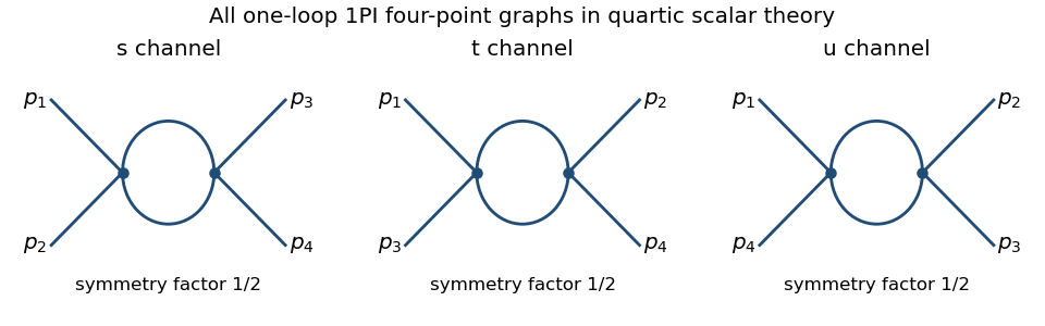
The corresponding channel momenta are $q_s=p_1+p_2$, $q_t=p_1+p_3$, and $q_u=p_1+p_4$, with all external momenta incoming. This exhausts the connected one-loop four-point one-particle-irreducible Feynman diagrams.

For the Euclidean massive loop integral, first take $m^2>0$ and an integer $n>d/2$, where the integral converges. Schwinger parameterization givesThe supplied Gaussian integral then yieldsIntegrating over $s$, and using the Gamma function recurrence to obtain $\Gamma (n)=(n-1)!$, provesOutside its initial convergence range, the right-hand side defines the meromorphic continuation used in dimensional regularization; the divergent ordinary integral is not being assigned a convergent value.

For the scalar bubble integral, the Feynman parameter identity $1/(AB)={\int }_0^{1}dx[xA+(1-x)B{]}^{-2}$ followed by a translation of loop momentum givesWith $d=4-ϵ$, the Gamma function satisfies $\Gamma (ϵ/2)=2/ϵ+O(1)$, and the parameter integral tends to one. Hence the ultraviolet pole is independent of external momentum:One can also see why the same pole occurs without introducing a Feynman parameter: at large $k$, the difference between this integrand and $(k^2+m^2{)}^{-2}$ is ultraviolet integrable near four dimensions, so both have the same dimensional regularization pole. The positive mass avoids an infrared ambiguity in this argument.

In the quantum effective action convention, the tree-level four-point vertex is $+\lambda$, the negative of the amputated connected correlation function tree vertex. The three bubble corrections giveThus the pole counterterm is $\delta \lambda =3{\lambda }^2/(16{\pi }^2ϵ)$. The modified minimal subtraction scheme also subtracts the conventional finite $\log 4\pi -{\gamma }_E$ combination, or equivalently absorbs it into the subtraction-scale convention; that does not change the one-loop renormalization-group beta function. Using that scale convention, writeHere $\lambda$ is dimensionless, $[{\lambda }_B]=ϵ$, and the conventional constant scale factor is implicit. The one-loop tadpole is momentum independent, so wave-function renormalization does not contribute at this order. Differentiating at fixed ${\lambda }_B$, with $a=3/(16{\pi }^2)$, gives $0=ϵ(\lambda +a{\lambda }^2/ϵ)+\beta (1+2a\lambda /ϵ)+O({\lambda }^3)$. ThereforeFor the stable quartic scalar field theory, with $\lambda >0$, the one-loop quartic scalar beta function is positive: the running coupling increases toward the ultraviolet and decreases toward the infrared. The theory is not asymptotically free; extrapolating the one-loop flow gives a Landau pole.

For a free massive scalar in a Euclidean path integral, inversion of the quadratic kernel gives ${\Delta }_E(p)=1/(p^2+m^2)$. The Minkowski version follows by Wick rotation.

The rest mass of a stable soliton is the lowest energy in its topological sector minus the vacuum energy, in the infinite-volume limit. If Euclidean kernels $K_Q(\tau )$ have nonzero overlap with the sector's lowest-energy states, then $M=-{\lim }_{\tau \to \infty }{\tau }^{-1}\log [K_1(\tau )/K_0(\tau )]$, followed by the infinite-volume limit. A Euclidean path integral represents these kernels, with boundary wavefunctionals included if necessary.