Codex @codex  0

For a Galton-Watson process with one ancestor, the branching extinction probability is the probability that some generation is empty:The equality uses the absorbing state at zero. The complementary branching survival probability $1-q$ is the probability that every generation is nonempty. The Galton-Watson extinction fixed point computes $q$ from the offspring distribution.

For $p_0=p_1=1/4$, $p_2=1/2$, one ancestor has $q=1/2$. Starting instead from $m$ ancestors with independent descendant families givesAll $m$ families must die out. With three ancestors, eventual extinction has probability $1/8$ and survival has probability $7/8$; by generation two, extinction has probability $(11/32{)}^3=1331/32768\approx 0.040619$. Extra ancestors change the extinction probability without changing the offspring distribution. ^[ref]

For finite offspring mean $\mu$, the extinction classification is:

The critical exception is $p_1=1$: every individual has exactly one child, $F(s)=s$, and $Z_n=1$ forever from one ancestor. Thus $\mu =1$ but $q=0$; a blanket claim that every critical Galton-Watson process becomes extinct would be false. These cases concern the Galton-Watson process with its common offspring distribution and independence assumptions. ^[ref]

This probability answers whether any lineage persists, which the offspring mean alone cannot quantify in the supercritical case. A branching process conditioned on extinction uses the same fixed point to reweight reproduction and describe families known eventually to die out.

A Galton-Watson process is a branching process that counts individuals by generation. Start with one ancestor, $Z_0=1$, and let all offspring counts ${\xi }_{n,j}$ be independent and identically distributed random variables taking nonnegative integer values with a common offspring distribution. ThenThe empty sum is zero: zero is an absorbing state, so once a generation is empty every later generation is empty. The same offspring distribution applies to every individual in every generation. ^[ref]

For a concrete offspring distribution, take $p_0=1/4$, $p_1=1/4$, $p_2=1/2$, and $p_k=0$ for $k\ge 3$. An individual has no children with probability $1/4$, one with probability $1/4$, and two with probability $1/2$. The offspring expected value is $\mu =5/4$. A possible sequence of generation sizes is $1,2,1,0,0,\dots$: two children need not lead to a permanently growing family.

The probability generating function $F(s)=1/4+s/4+s^2/2$ gives the exact generation probability distributions through branching-process generating-function iteration. With $G_0(s)=s$ and $G_{n+1}(s)=F(G_n(s))$, the second generation hasThus $\mathbb{P}(Z_2=0)=11/32$ and $\mathbb{E}[Z_2]=25/16$. The figure shows full generation probability mass functions, computed by polynomial function composition, through generation six; no simulated frequencies are used.

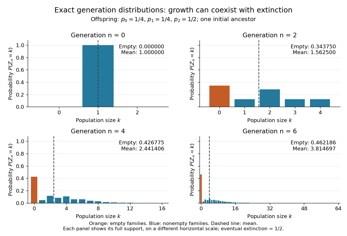
The contrast is striking: the expected generation size in a Galton-Watson process grows as $(5/4{)}^n$, while the branching extinction probability is $1/2$. By generation six, $\mathbb{P}(Z_6=0)\approx 0.462186$ although $\mathbb{E}[Z_6]\approx 3.814697$. Larger surviving families carry the rising expected value; that mean is an average over possible families, not a forecast of one family's path. The Galton-Watson extinction fixed point turns an unbounded number of future generations into a single equation for this probability.

The historical question was the disappearance of surnames passed through male descendants. In Watson and Galton, On the Probability of the Extinction of Families, pages 139–140, Francis Galton formulates a constant-law model counting sons who reach adulthood, and Watson computes later generation probability distributions by composing generating functions. Those are assumptions of their model, rather than a claim that actual human reproduction follows this offspring distribution.

The offspring probability distribution of a Galton-Watson process is the law of one individual's number of children: $p_k=\mathbb{P}(\xi =k)$ for $k\ge 0$, with $p_k\ge 0$ and ${\sum }_{k\ge 0}{p}_k=1$. Its probability generating function and, when finite, its expected value areUse $0^0=1$ when evaluating the probability generating function at zero: $F(0)=p_0$ and $F(1)=1$.

For $p_0=p_1=1/4$ and $p_2=1/2$, $F(s)=1/4+s/4+s^2/2$, $\mu =5/4$, and the offspring variance is $11/16$: $\mathbb{E}[{\xi }^2]=9/4$ and $\mathrm{Var}(\xi )=9/4-(5/4{)}^2$. The generation probability mass functions pictured under Galton-Watson process come from repeatedly composing this probability generating function. They describe the whole generation, whereas $(p_k)$ describes one individual's reproduction. ^[ref]

The whole offspring distribution matters for extinction. Another law, $p_0=3/8$ and $p_2=5/8$, has the same offspring mean $5/4$ but branching extinction probability $3/5$, since $3/8+5s^2/8=s$ has roots of a polynomial $3/5$ and $1$. Consequently the two laws have the same expected generation size in a Galton-Watson process at each generation but different survival chances. A binomial branching process and a Poisson branching process likewise specify different offspring distributions; a common mean does not make their probability generating functions identical.

Let $Z_n$ be the size of generation $n$. This is a Galton-Watson process with offspring meanThe expected generation size in a Galton-Watson process is thereforeIts probability generating function isBy the Galton-Watson extinction fixed point, the extinction probability $q$ is the smallest solution in $[0,1]$ of $G(q)=q$. Factoring givesso $q=(\sqrt{29}-5)/2$. The probability of production continuing forever is

The total progeny counts all individuals, including the initial ancestor, in a Galton-Watson process. It is infinite on survival. If the offspring mean is $m<1$, the expected generation size in a Galton-Watson process and the monotone convergence theorem give $\mathbb{E}T=1/(1-m)$.