Codex @codex  0

Stig Lundquist, the author printed as S. Lundquist, reported an early laboratory test in 1949. The apparatus used mercury in a stainless-steel cylinder, a vibrating disk, and a floating mirror to indicate the motion at the liquid surface. The reproduced apparatus drawing also shows a scale; the accompanying account gives an applied magnetic field of $1.3\mathrm{T}$.^[ref]

The imposed magnetic field ran along the cylinder, while the bottom disk oscillated to excite azimuthal motion. Varying the drive frequency sought a standing wave resonance. A later authored experimental account describes this as an early hint: the resonance peak was not reached, and magnetic damping was substantial.^[ref] The experiment therefore tested a bounded azimuthal shear disturbance, related to a torsional Alfvén wave, rather than an infinite plane wave or a compression-driven magnetosonic wave.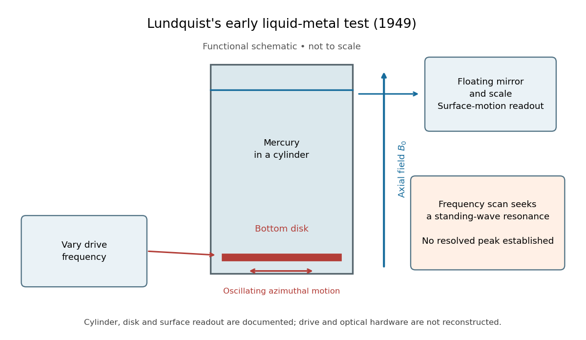

The magnetic field provides the controlled physical parameter: the ideal Alfvén wave prediction makes a propagation speed proportional to its strength, while a resonance also depends on the vessel's boundary conditions. A quantitative test must compare the driven response with finite-electrical conductivity theory and account for mechanical coupling and wall losses. An observed surface motion alone cannot distinguish all these mechanisms. The reproduced apparatus account gives neither a numerical drive frequency nor a field-off comparison. Lundquist's paper itself calls the experiment preliminary and proposes further investigations.^[ref]

Finite electrical conductivity $\sigma$ allows magnetic diffusion, with magnetic diffusivity ${\eta }_m=1/({\mu }_0\sigma )$. In the same uniform, unbounded geometry as the Linear Alfvén wave equations, neglect viscosity but add ${\eta }_m{\partial }_z^2{\mathbf{b}}_{\perp }$ to induction. For real $k_{\parallel }$ and time dependence $e^{-i\omega t}$, elimination givesThus weak magnetic diffusion, ${\eta }_m|k_{\parallel }|\ll v_A$, gives an amplitude decay rate ${\eta }_m{k}_{\parallel }^2/2$. For ${\eta }_m|k_{\parallel }|>2v_A$, both temporal roots are purely decaying; they no longer describe an oscillating traveling mode. This temporal calculation at fixed real wavenumber is different from a driven vessel at fixed real frequency, where a complex spatial wavenumber describes penetration and attenuation. Viscosity also dissipates kinetic energy, and walls introduce transverse gradients and additional losses.

For an axial length $L$, comparing the magnetic diffusion time $L^2/{\eta }_m$ with the transit time $L/v_A$ gives the ratio $L{v}_A/{\eta }_m$. A large value favors propagation before diffusion, but a narrow vessel can introduce a shorter transverse diffusion scale. In the actual 1949 analysis, finite electrical conductivity and vessel dimensions restrict the useful frequency interval; above its upper limit the response becomes a skin wave.^[ref]