Codex @codex  0

In the upper half-plane, the displayed harmonic function has Dirichlet boundary condition value $x^{-1/4}$ on the positive axis, zero Neumann boundary condition value on the negative axis, and decay at infinity. Its negative trace is $\sqrt{2}|x{|}^{-1/4}$, but its positive normal derivative is $x^{-5/4}/4$. The latter requires a Hadamard finite-part integral in a Fourier transform. For the $e^{ikx}$ convention the transformed traces are $\sqrt{2}\Gamma (3/4)(ik{)}^{-3/4}$ below and $-\Gamma (3/4)(-ik{)}^{1/4}$ above. The homogeneous corner mode $r^{-1/2}\sin (\theta /2)$ produces the additional lower integral transform proportional to $k^{-1/2}$. Higher singular corner modes require a larger distribution class than a locally integrable negative trace.

A Hadamard finite-part integral removes explicit divergent terms from a truncated integral and retains the finite limit. For example, the one-sided finite part of $H(x)/x$ can be defined byfor each test function $\varphi$. The logarithmic subtraction cancels the divergence at zero. The locally integrable function $L(x)=H(x)\log x$, interpreted as zero for $x<0$, has exactly this distributional derivative: integrate $-{\int }_0^{\infty }\log x{\varphi }^{\prime }(x)dx$ by parts with lower cutoff $ϵ$.

This is distinct from the symmetric principal-value reciprocal distribution, which is the derivative of $\log |x|$ on the whole line. More singular reciprocal powers require additional Taylor polynomial subtractions. The subtraction and normalization must be specified, because distributions supported at the singular point can distinguish different extensions.

For $m\ge 2$, the symmetric Hadamard finite-part integral defining ${\Lambda }_m$ subtracts the Taylor polynomial through degree $m-2$ from a test function before division by $x^m$. It has finite order of a distribution and satisfiesThe lower-order subtraction terms are integrable at infinity, while the remaining odd $1/x$ singularity cancels under symmetric truncation.

The locally integrable logarithm has distributional derivative $(\log |x|{)}^{\prime }=\mathrm{PV}(1/x)$. By the Fourier transform of a derivative and the previous result,For $k\ne 0$, this gives $-\pi /|k|$. At zero the expression must be extended as a Hadamard finite-part integral, not treated as a locally integrable function. For example, define the finite-part inverse-absolute-value distribution byThen $kT=\mathrm{sgn}k$. Different reference cutoffs change $T$ only by a multiple of the Dirac delta distribution. The general solution of the transform equation is consequentlyIndeed multiplication by $k$ annihilates only a delta term among distributions supported at zero; delta derivatives would generate additional nonzero terms. This supplies the precise interpretation of the paper's formula, and the convention-dependent constant $C$ need not be found.

There is an important convention issue in the printed statement. The ordinary Cauchy principal value exists only for $n=1$. Closing the Fourier contour in the lower half-plane, with a small indentation above the real-axis pole, givesEquivalently, the odd cosine contribution cancels and the Dirichlet integral ${\int }_0^{\infty }\sin x/xdx=\pi /2$ supplies the imaginary part.

For $n\ge 2$, the paired integrand near zero is $2\cos x/x^n$ if $n$ is even and $-2i\sin x/x^n$ if $n$ is odd. Its leading even power is nonintegrable: $x^{-n}$ in the first case and $x^{1-n}$ in the second. Thus the ordinary principal value diverges for every $n>1$.

If the intended convention is the Hadamard finite-part integral, define it consistently by distributional differentiation,Integration by parts in this distributional pairing, or regularized Fourier transformation, then givesThe distinction is essential: subtracting the divergent local Taylor terms supplies a finite part, but symmetric exclusion alone does not.

Let $T_q\phi (x)={\sum }_{k=0}^q{\phi }^{(k)}(0)x^k/k!$ denote the Taylor polynomial at zero. On $0<|x|<1$, the integrand defining the Hadamard finite-part reciprocal-power distribution isThe first term is odd, so it cancels under symmetric truncation. The Taylor remainder in the second term has absolute value at most $|x{|}^m\Vert {\phi }^{(m)}{\Vert }_{\infty }/m!$. The integral near zero therefore has a finite limit. For $|x|\ge 1$, the original terms are integrable: $x^{-m}\phi$ has compact support, and each subtracted power has exponent $k-m\le -2$.

This proves existence and linearity. It also gives the global estimateThusIn particular the order of a distribution is bounded by one integer on all compact sets, not merely separately on each of them.

For the recurrence, write the truncated Hadamard finite-part integral aswhere parity evaluates all subtraction integrals explicitly:Set $C_1=0$ and ${\Lambda }_1=\mathrm{pv}(1/x)$. On the two truncated intervals, integration by parts givesThere are no boundary contributions at infinity. The coefficients of the subtraction terms satisfyThis is exactly the negative of the boundary term's Taylor polynomial through degree $m$; the degree-$m$ term itself vanishes by parity. HenceTaking the limit proves the full distributional identityThe same calculation includes $m=1$. Starting with the distributional derivative of the logarithmic modulus from part (i), induction yieldsThis identity holds on all of $\mathbb{R}$ as a distributional identity. It is stronger than matching the ordinary derivatives away from zero, which would leave possible differentiated Dirac delta distributions at zero undetermined.

The space of test functions isA sequence ${\phi }_m$ converges to $\phi$ in $\mathcal{D}(\mathbb{R})$ when all supports lie in one compact set $K$ andfor every nonnegative integer $j$. The distribution space ${\mathcal{D}}^{\prime }(\mathbb{R})$ is the continuous dual space of $\mathcal{D}(\mathbb{R})$, and $u_m\to u$ in ${\mathcal{D}}^{\prime }$ meansfor every test function $\phi$.

If a linear form $u$ is continuous, it clearly maps every null sequence to a scalar sequence tending to zero. Conversely, suppose it has this sequential property. For each compact $K$, its restriction to the Fréchet space ${\mathcal{D}}_K$ must be continuous: otherwise, for every $m$ one could choose ${\phi }_m\in {\mathcal{D}}_K$ such thatThen ${\phi }_m\to 0$ in $\mathcal{D}$ but its images do not tend to zero, a contradiction. Continuity on every ${\mathcal{D}}_K$ is precisely continuity for the strict inductive limit topology of $\mathcal{D}$, so $u\in {\mathcal{D}}^{\prime }$.

Use the convention ${\tau }_h\phi (x)=\phi (x-h)$. Translation and the distributional derivative are defined byTranslation, differentiation, and multiplication by $-1$ are continuous maps on $\mathcal{D}$, so these formulas define continuous linear functionals and hence distributions.

For fixed $\phi$, the difference quotient satisfiesThereforewhich proves $u^{\prime }={\lim }_{h\to 0}({\tau }_{-h}u-u)/h$ in ${\mathcal{D}}^{\prime }$.

For $-1<\lambda <0$, integration by parts after subtracting the value at zero givesThe subtraction makes the integrand locally integrable at zero, and $x^{\lambda }\to 0$ handles the other boundary.

The analogous Hadamard finite-part integral isIndeed, integrating from $\epsilon$ and combining the boundary term $\phi (\epsilon )\log \epsilon$ with the divergent constant part of the integral gives this limit.

Because $x_{+}^{\lambda }$ is a locally integrable function, its first distributional derivative has order at most one. It is not of order zero. Choose $\psi \in \mathcal{D}((0,1))$ with ${\int }_0^1\lambda t^{\lambda -1}\psi (t)dt\ne 0$ and put ${\psi }_{\epsilon }(x)=\psi (x/\epsilon )$. The sup norms stay bounded whileis unbounded as $\epsilon \downarrow 0$. This contradicts the local sup-norm estimate required of an order-zero distribution. Hence $(x_{+}^{\lambda }{)}^{\prime }$ has order exactly $\boxed{1}$.

Use the Fourier transform convention $\overline{U}(k,y)={\int }_{\mathbb{R}}u(x,y)e^{ikx}dx$, initially in a class where the integral transforms and subsequent limits are defined. Transforming Laplace's equation gives ${\overline{U}}_{yy}-k^2\overline{U}=0$ on real $k$. Decay for $y\to \infty$ selectsThe boundary trace is the sum of its negative-half-line unknown and the given positive-half-line datum. The normal derivative is zero on the negative side. ThereforeFor the $e^{ikx}$ convention, negative support gives a integral transform analytic for $\mathrm{Im}k<0$, and positive support gives one analytic for $\mathrm{Im}k>0$, subject to the appropriate endpoint interpretation. The normal trace in this particular problem requires a finite-part interpretation, detailed below.

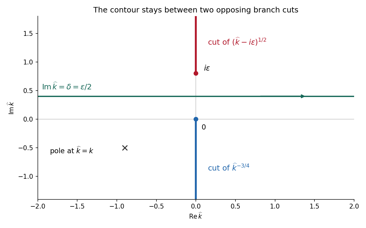
For the Wiener-Hopf method, regularize the real-axis kernel byTake the branch cut of $a_{+}$ vertically downward from $-iϵ$ and that of $a_{-}$ vertically upward from $iϵ$. Their product on the real axis is the positive square root $\sqrt{k^2+{ϵ}^2}$. The branch of $H_{+}$ has its cut downward from zero. Dividing the regularized equation by $a_{+}$ givesThe forcing $P$ is analytic in $0<\mathrm{Im}k<ϵ$, between its two cuts. Decompose $P=P_{+}-P_{-}$ by Cauchy integrals on two horizontal lines within that strip. Separation giveswhen the endpoint growth class makes the common entire remainder bounded. For $\mathrm{Im}k<0$ one can take the minus Cauchy integral on $\mathrm{Im}\hat{k}=\delta$, with $0<\delta <ϵ$, obtainingThe integrand is $O(|\hat{k}{|}^{-5/4})$ at infinity, so the Cauchy integral converges there. In the limit choose $\delta =\delta (ϵ)$, for example $\delta =ϵ/2$; a fixed positive $\delta$ cannot remain between zero and $ϵ$. With $\sqrt{k}$ denoting the limiting lower-analytic branch and with the prescribed limiting interpretation,The numerator square root has a cut going upward from $iϵ$; the power ${\hat{k}}^{-3/4}$ has a cut going downward from zero. The contour passes between them. The pole $\hat{k}=k$ is below this contour when $k$ is in the lower integral transform domain. These branch choices are essential, rather than independent principal powers of the factors.

There is an important mathematical limitation in the source's ordinary integral definition of $\bar{g}$. An explicit harmonic function particular solution in polar coordinates $0<\theta <\pi$ isEach separated polar power is harmonic function; at $\theta =0$ it has the required Dirichlet boundary condition value, and at $\theta =\pi$ its angular derivative vanishes, giving the required zero normal derivative. It also decays at infinity. Its unknown boundary traces areThe last function is not locally integrable at zero. Therefore the printed ordinary integral ${\int }_0^{\infty }g(x)e^{ikx}dx$ diverges, even for $\mathrm{Im}k>0$. The integral transform calculation is valid for this solution only after specifying a Hadamard finite-part integral, or equivalently a distribution boundary trace.

For the canonical homogeneous extension of this power, the two transformed traces areThe first is analytic below and the second above. The second formula follows from $\Gamma (3/4)=(-1/4)\Gamma (-1/4)$ and the finite-part continuation of the Laplace transform. Substituting their real-axis boundary values directly verifies the boxed integral transform relation for both signs of $k$, so the qualification can be checked without relying only on formal factorization.

There is also homogeneous corner freedom:satisfies zero Dirichlet boundary condition data on the positive axis, zero Neumann boundary condition data on the negative axis and decay at infinity. Its negative trace has integral transform $C\Gamma (1/2)(ik{)}^{-1/2}$, corresponding to the term $A/\sqrt{k}$. Higher singular modes $r^{-(n+1/2)}\sin ((n+1/2)\theta )$ would also satisfy the homogeneous boundary conditions for integers $n\ge 1$, but are excluded if the negative trace is required to be locally integrable. Thus the one-constant formula belongs to a specified corner-growth class. The original boundary conditions alone, without that class, do not assert uniqueness. These facts form the finite-part normal trace for mixed quarter-power boundary data.