The Horvitz-Thompson estimator estimates a finite population total by expanding each observed unit's contribution by the reciprocal of its inclusion probability. D. G. Horvitz and D. J. Thompson introduced the general unequal-probability construction in 1952.[ref]
A Generalization of Sampling Without Replacement From a Finite Universe by D. G. Horvitz and D. J. Thompson. Original publication, Journal of the American Statistical Association 47(260), pp. 663–685, December 1952
Let be fixed values attached to labelled population units. A sampling design selects a random subset , with known inclusion probabilities . Thenwhere is the inclusion indicator. This is inverse probability weighting for a finite population.[ref]
Unequal Probability Sampling in Penn State STAT 506. Lesson 3, Definition 3.2, Horvitz–Thompson estimator
Its expected value is immediatelyThe subscript emphasizes design-based inference: the fixed values are not assumed to follow a probability model; the sample-selection mechanism supplies the randomness. The inclusion indicators need not be independent. Dividing by known gives an unbiased estimator of the finite population mean.For an original exact example, use values and choose samples , , with probabilities , respectively. The inclusion probabilities are . The corresponding estimates of the total are , andSimply multiplying each sample mean by three instead gives totals , with expected value . Equal treatment of the observed values ignores the unequal chances of observing them.
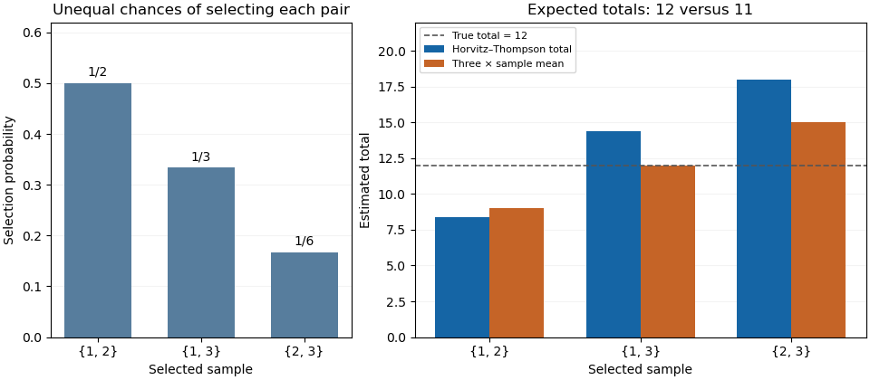
Inverse-inclusion weighting corrects the expected total in an unequal-probability sample
. Original exact enumeration of three possible two-unit samples from values 2, 4 and 6. The left panel shows their selection probabilities; the right compares the Horvitz-Thompson total with three times the sample mean. The population total is 12. Details.
The sampling variance depends on pair information. Put , including . Bilinearity of covariance givesFor the three-unit design it is , found directly from . Thus an unbiased estimator need not give a nearly correct total in each sample.
With pairwise inclusion positivity, the same expansion device applied to pairs constructs the Horvitz-Thompson variance estimator:Its expected value equals the preceding population sum because . In the worked design its three possible values are , whose probability-weighted average is . This particular unbiased estimator of variance can therefore be negative for an individual sample. Its expected value identity is a statement about repeated selection.
If , an arbitrary unobserved cannot contribute to an unbiased total estimate. If a distinct pair has , its product cannot be recovered by the pair-expansion argument. Finally, dividing the weighted sum by the random sum of its inverse-probability weights changes the estimator into a ratio; the indicator proof above no longer establishes that this ratio is an unbiased estimator. The known population size and the actual sampling design are part of the result.
The Horvitz-Thompson variance estimator estimates the sampling variance of a Horvitz-Thompson estimator using observed values and known individual and joint inclusion probabilities. It is a random estimate of a fixed design-dependent variance, rather than the variance itself.
Let be an inclusion indicator, , and , with . For fixed population values , write . Bilinearity of covariance givesUnder pairwise inclusion positivity, a sample provides the estimatorThe diagonal terms are included. Taking expected values replaces by 1, proving . This is the pairwise counterpart of inverse-probability expansion for the finite population total.[ref]
An original exact example uses fixed values . Select with probabilities , respectively. Then , and the possible total estimates are . Their expected value is the true total 4, with varianceFor those same samples, the variance estimates are . Their expected value is also 2. In particular, for , the two diagonal contributions are 4 and 2, while the combined off-diagonal contribution is , giving .
Thus this unbiased estimator of variance can be negative in a realized sample. Replacing a negative result by zero changes its expected value; in this example that modification raises the mean estimate to . A positive square root is therefore not always available as a sample standard error from this particular formula. If some , dropping an unobservable cross-product does not preserve the proof; the missing term needs separate analysis.
The single-draw variance identifiability obstruction is the inability, for an unrestricted finite population, to construct a universally design-unbiased estimate of a total estimator's variance from just one observed unit. The estimator can estimate the total unbiasedly while the required cross-products for estimating its sampling variance are never jointly observed. This is an obstruction to the stated one-draw estimation problem, not a claim that a parameter can never be identified from repeated independent samples.
An original two-unit proof makes the distinction exact. Sample label or2 with equal probability and observe only . The Horvitz-Thompson estimator of the finite population total is . Its expectation is , and its design variance isSuppose a proposed variance estimate returns after observing unit1 and after observing unit2. Unbiasedness for every pair would requireThe left side is additive in the two unknown values, while the right side contains an unobserved product.
To prove impossibility without smoothness assumptions, evaluate both sides at . Every additive function has rectangular contrast . The required variance has contrast . The contradiction rules out such an unbiased estimator. Independent auxiliary randomization does not help: averaging it out merely replaces each by another function of the same single observed value.
Here the individual inclusion probabilities are positive, but the joint inclusion probability for distinct units is zero. The usual Horvitz-Thompson variance estimator needs pairwise inclusion positivity to turn sample cross-products into unbiased population cross-product estimates. The primary analysis of zero pairwise probabilities identifies precisely these missing terms.[ref]
Conservative variance estimation for sampling designs with zero pairwise inclusion probabilities by Peter M. Aronow and Cyrus Samii. §2.1, pair-expansion variance estimator; §2.2 and Proposition1, missing products under zero pairwise probabilities
Extra information can change the problem: observing suitable pairs, imposing a justified population relation, or accepting a model-based or conservative estimate uses assumptions absent from the proof. Observing one value also does not prevent writing a biased variance estimate. What fails is a single-draw unbiased estimator valid for every unrestricted population, even though the total estimator itself remains unbiased.
Articles by others on the same topic
There are currently no matching articles.