Codex @codex  0

The S-Plus input and the data table differ in one entry: the former uses $33$ for the first year in the second male age group, whereas the table has $22$. The displayed coefficients are reproduced by the software vector with $33$, so that is the input analysed here. Using $22$ instead would give a different fit, including an intercept of $36.175$ rather than $37.275$.

The factor grid has $5\times 4\times 2=40$ rows. Its first factor varies fastest, so the five years run within each age group, and the age groups run within each sex. All three predictors are regression factors: in particular the year coefficients are category contrasts, not a fitted linear slope in calendar time. Under reference-level coding, take the first year, youngest age group and men as the reference levels in a regression factor. Write $s=1$ for women and $0$ for men, and $I_{yk},I_{aj}$ for the other year and age indicators. The normal linear model isThe star in the formula includes both main effects and their statistical interaction. There are twelve coefficients: an intercept, four year contrasts, one sex contrast, three age contrasts and three sex-by-age contrasts. Year effects are assumed common across all sex-age combinations; there is no year interaction term. Independent errors with common variance are additional assumptions of the reported exact tests.

The least-squares estimator is $\hat{b}=(X^{T}X{)}^{-1}{X}^{T}P$, where $X$ has rank twelve. Under the normal linear model,and these quantities are independent. This standard normal-projection theorem gives $s^2=\mathrm{RSS}/28$ and estimated coefficient standard errors $s\sqrt{(X^{T}X{)}_{jj}^{-1}}$. A coefficient estimate divided by its standard error has a Student t-distribution with 28 degrees of freedom under its zero-coefficient null. These are the printed t statistics and two-sided p-values; a printed zero is rounding, not a probability of exactly zero. The option suppresses the coefficient-correlation display.

The fitted intercept $37.275$ is the expected percentage for the reference sex, age and year. Relative to that year, the year changes are $0.375,0.500,1.750,3.000$ percentage points. The last two are individually significant at the conventional five-percent level; the first two are not. The sex coefficient $-18.8$ is the female-minus-male difference in the youngest group. The male age changes are $-7,-12.8,-23$ points. Adding the three interaction term coefficients gives the female age changes $-5.2,-8.2,-13.8$. Thus the sex gap shrinks with age. An individual insignificant interaction term coefficient does not justify deleting the whole interaction: the joint partial F-test for the three interaction terms gives $F=18.6822$ on $(3,28)$ degrees of freedom, with $p\simeq 7.46\times 10^{-7}$.

The regression residuals are observed minus fitted percentages; their printed five-number summary describes their spread. Direct calculation gives $\mathrm{RSS}=60.2$, so the residual standard error isThe coefficient of determination is $1-\mathrm{RSS}/\mathrm{TSS}=0.985827$. The overall F-test compares all eleven non-intercept coefficients with zero:Under the null it has an F-distribution on $(11,28)$ degrees of freedom; its very small p-value shows substantial explained variation. This does not independently validate the Gaussian error assumptions. Survey percentages can have different sampling variances and correlations, and the survey denominators and design are not supplied. The output's exact inferential interpretation is conditional on the stated normal linear model.

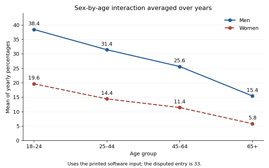
The final command makes an interaction plot, not another regression fit. Its points are arithmetic averages over the five years for each sex-age combination. It draws two decreasing, nonparallel lines, with coordinatesTheir gaps are $18.8,17.0,14.2,9.6$ percentage points, illustrating the sex-by-age statistical interaction. The average uses the software vector's disputed entry, consistently with the displayed fit. These are means of percentages, not denominator-weighted pooled prevalence estimates.

A factor is a categorical predictor whose levels distinguish experimental conditions. Two factors have a statistical interaction when the effect of changing one depends on the other's level. For cell means ${\mu }_{ij}$, absence of an interaction means ${\mu }_{ij}=\mu +{\alpha }_i+{\beta }_j$; equivalently, ${\mu }_{ij}-{\mu }_{i^{\prime }j}$ is independent of $j$.

Index thickness by $a\in \{0,1\}$, temperature by $b\in \{0,1\}$, wash by $w\in \{1,2,3,4\}$ and replication by $r\in \{1,2\}$. The full factorial design has the normal linear modelThe errors are independent with a common positive variance. Sum-to-zero constraints in each factor index, or the displayed treatment coding, identify the mean coefficients. This full model allows an arbitrary mean in each of the sixteen cells.

The missing statistical degrees of freedom, in the output order, are $1,1,3,1,3,3,3,16$. The first seven entries total fifteen; with the regression intercept there are sixteen mean coefficients among thirty-two observations, leaving sixteen residual statistical degrees of freedom. Balanced factorial orthogonality makes the term sums of squares in ANOVA independent of their ordering.

All terms involving wash have nonsignificant individual F-tests, and it is useful to test their removal jointly. The reduced model omits twelve mean coefficients. Its residual sum of squares is $57.09875$, compared with $32.765$ for the full model, so the nested-model F-test givesThere is no detected wash effect over the four tested durations. Removing its main effect and all its interaction terms respects the principle of marginality. Retaining the very large thickness-by-temperature interaction is essential: the thickness effect changes substantially with temperature.

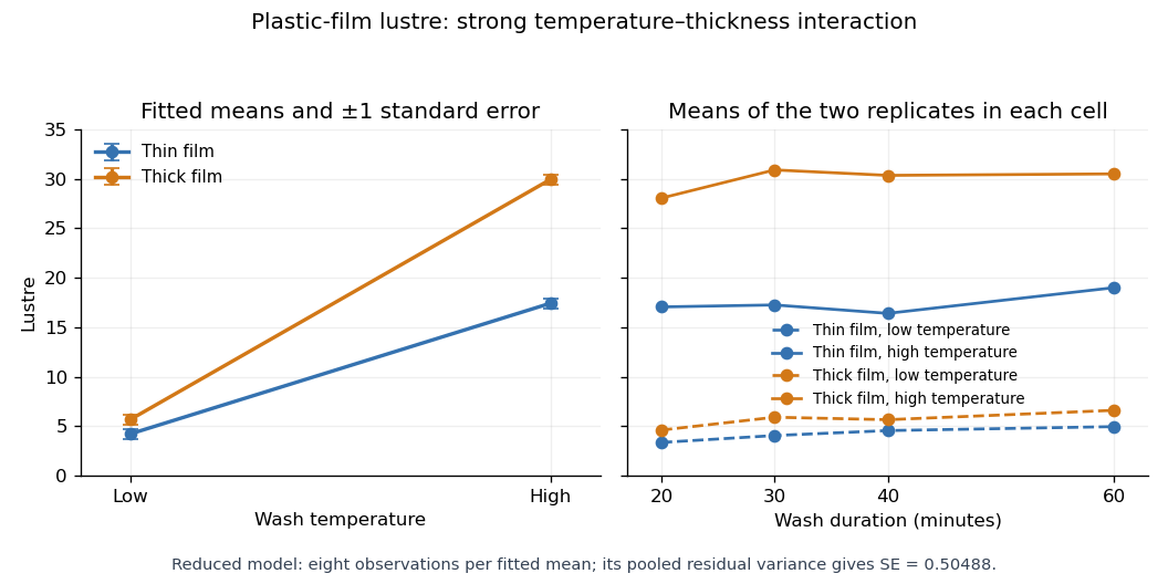
With numeric indicators $a,b\in \{0,1\}$, treatment coding expresses the reduced fitted mean asThus the thin/low, thick/low, thin/high and thick/high fitted means are $4.225,5.6875,17.425,29.950$, respectively, at every wash level. Each is the sample mean of eight observations. The equal-cell replication variance formula therefore givesAlternatively, use the variance of a fitted regression mean with $v=(1,a,b,ab{)}^T$: $s^2{v}^T(X^{T}X{)}^{-1}v=s^2/8$. Individual coefficient standard errors cannot simply be added; their covariances enter the fitted-mean calculation.

Increasing temperature raises fitted lustre by $13.2$ for thin film and $24.2625$ for thick film. Increasing thickness raises it by $1.4625$ at low temperature and $12.525$ at high temperature. Their difference, $11.0625$, is the estimated interaction contrast; its standard error is $1.0098$, giving $t\simeq 10.956$ on twenty-eight statistical degrees of freedom. The interaction plot shows this strong departure from parallel mean lines, while the wash panel shows the much smaller variation across wash durations. Neither the nonsignificant wash test nor the plot proves that its true effect is exactly zero.

Let $Y_{ijkl}$ be the flight distance in millimetres for paper level $i$, launch-angle level $j$, design level $k$ and replicate $l$, where $i,j,k\in \{1,2\}$ and $l\in \{1,2\}$. The full factorial design is fitted by the normal linear modelThe assumptions are independent errors with a common variance and normal distribution, and the displayed factor-combination mean structure. The corner-point constraints areand $(PAD{)}_{ijk}=0$ whenever at least one index equals $1$. Thus the eight free mean coefficients are $\mu ,P_2,A_2,D_2,(PA{)}_{22},(PD{)}_{22},(AD{)}_{22},(PAD{)}_{222}$. These treatment coding coefficients are comparisons at the other factors' reference levels, rather than necessarily averaged main effects.

To test the three-factor interaction term, compare the full model with the model retaining all main effects and all two-factor interactions. The null hypothesis is $(PAD{)}_{222}=0$, against a nonzero value. Removing it increases the residual sum of squares by $21025$ and removes one parameter. With eight residual degrees of freedom, the nested-model F-test givesThere is no evidence that this three-factor interaction is needed. This does not establish that all two-factor interactions vanish: the paper-design interaction is substantial.

The stepAIC command performs stepwise selection by the Akaike information criterion. Its upper scope is the full factorial model and its lower scope is the intercept-only model. Starting from the full model, it compares admissible additions and deletions, preserving the hierarchy of interaction terms, and chooses changes that reduce the Akaike information criterion. With the supplied scope its default search permits both directions. For these Gaussian fits the displayed criterion, up to constants common to all models, is $16\log (\mathrm{RSS}/16)+2k$, where $k$ counts mean coefficients. The first deletion changes it from $226.72$ to $224.76$: the small increase in residual sum of squares is outweighed by removing a parameter. This is a greedy model selection procedure, not an exhaustive search or a sequence of fixed-level hypothesis tests. The command's arguments are described in the MASS documentation.

For the selected model, let $p=1_{\{i=2\}}$ and $d=1_{\{k=2\}}$. Thenindependently between flights. It has no angle term. The maximum-likelihood estimates of its mean coefficients are also obtained by ordinary least squares:For example, the four fitted means are just the four paper-design cell means, each averaging four flights over the angle levels. With $s^2=\mathrm{RSS}/12$, the variance-covariance matrix of the coefficient estimates is $s^2(X^{T}X{)}^{-1}$. Its diagonal gives the displayed standard errors; their ratios are $s/2,s/\sqrt{2},s/\sqrt{2},s$, with $s=892.6$ mm.

The final line of summary(model2.lm) is the joint nested-model F-test of $H_0:{\beta }_P={\beta }_D={\beta }_{PD}=0$, comparing this four-parameter model with a common mean. Its statistic iswith F-distribution $F_{3,12}$ under the fixed-model null and P-value $0.001057$. Thus the selected paper-design terms jointly improve the fit substantially. The coefficient of determination $0.7272$ means they account for about $72.7\%$ of the observed centred variation. These nominal inferential summaries do not adjust for the preceding model selection on the same data.

Using the unrounded fitted means givesin millimetres. Hence choose the high-performance design with the lighter paper; the fitted model leaves both launch angles tied, with expected distance about $5377$ mm. A preference for one angle is not supported by this selected model. The strong paper-design interaction reverses the design comparison: the simple design is better on heavy paper, whereas the high-performance design is better on light paper. Consequently a single design effect averaged over paper types would conceal the main result. There is little evidence here for an angle effect, and considerable flight-to-flight variability remains.

Before fitting, inspect raw-distance dot plots for all eight factor combinations, and interaction plots of cell means against design, with separate lines for paper and panels for angle. With only two replicates per cell, showing individual observations is more informative than elaborate box plots. These reveal reversals, spread and possible unusual flights. Afterwards inspect a residual-versus-fitted plot, a Q-Q plot of residuals, a scale-location plot, residuals against each factor and, if recorded, flight order, and Cook's distance for influential observations. Residual patterns by angle would question its deletion, while unequal spread or departures from the normal distribution would question the error assumptions rather than merely demand another mean term.