Codex @codex  0

Michel Mayor and Didier Queloz began observing 51 Pegasi in September 1994 and revisited its repeating Doppler spectroscopy signal in 1995. Their circular fit used 35 measurements: orbital period $4.2293\pm 0.0011$ days, stellar radial-velocity semi-amplitude $59\pm 3\mathrm{m}{\mathrm{s}}^{-1}$, and residual scatter $13\mathrm{m}{\mathrm{s}}^{-1}$ after epoch-dependent velocity offsets. Apparently stable comparison stars checked the instrumental zero point. Low chromospheric stellar activity and an inferred roughly 30-day stellar rotation period argued against starspots; light curves and the spectral line bisector tested stellar pulsation. These checks favoured orbital motion but had finite sensitivity. The reported $M_p\sin i=0.47\pm 0.02$ Jupiter masses was not a true mass. Stronger upper bounds used stellar-spin information and assumed spin–orbit alignment, limiting a nearly face-on binary star interpretation conditionally.^[ref]

The hot Jupiter matters both for planetary migration and for how exoplanets are found. At fixed small companion mass, orbital inclination and orbital eccentricity, the stellar radial-velocity semi-amplitude scales as $K\propto P^{-1/3}$. Comparing chosen orbital periods of $4$ days and $12$ years gives an amplitude ratio of about $10.3$: a close companion can be much easier to detect and complete many orbits during one observing season. Finding a giant planet close to its star also asks how its present orbit relates to where it formed. Doppler spectroscopy supplies a dynamical constraint; it does not by itself establish a formation pathway or measure the exoplanet's radius.

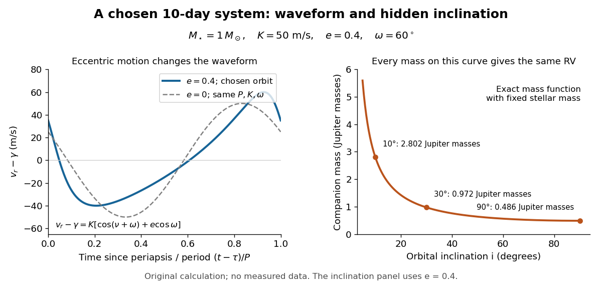
A repeating Doppler shift contains more than an amplitude. For an isolated two-body problem, let $\nu$ be the true anomaly, ${\omega }_{\star }$ the stellar argument of periapsis, $\tau$ the periapsis time and $\gamma$ the constant system line-of-sight velocity. The companion's argument of periapsis differs by $\pi$ from ${\omega }_{\star }$, so mixing the two conventions reverses the orbital signal. With positive velocity for recession, choose the stellar line-of-sight coordinate positive away from the observer. Kepler's equation supplies the clock:Here $M$ is the mean anomaly and $E$ the eccentric anomaly. The time coordinate is uniform in $M$, not in $\nu$: an eccentric Kepler orbit runs fastest near periapsis.

To derive the velocity law without guessing a sinusoid, write the stellar orbital coordinates as $X=a_{\star }(\cos E-e)$ and $Y=a_{\star }\sqrt{1-e^2}\sin E$. Project toDifferentiating $z$ and substituting the true anomaly identities givesThe constant $e\cos {\omega }_{\star }$ term makes the time average of the orbital velocity zero: $z$ returns to its original value after one orbital period. For $e=0$ this reduces to a sinusoid with an arbitrary phase origin; periapsis itself is then undefined. For $e>0$, the largest and smallest velocities are $\gamma +K(e\cos {\omega }_{\star }\pm 1)$, so $K$ is still half the peak-to-peak range, although the extrema need not be symmetric about $\gamma$.

For an original worked example, choose $M_{\star }=1M_{\odot }$, $P=10$ days, $K=50\mathrm{m}{\mathrm{s}}^{-1}$, $e=0.4$ and ${\omega }_{\star }=60^{\circ }$. Taking one day as $86400\mathrm{s}$ and $G=6.67430\times 10^{-11}{\mathrm{m}}^3\mathrm{k}{\mathrm{g}}^{-1}{\mathrm{s}}^{-2}$, the binary mass function is $f=1.98270\times 10^{20}\mathrm{kg}$. Its units check directly: $[P{K}^3/G]=\mathrm{kg}$. With adopted solar mass $M_{\odot }=1.98847\times 10^{30}\mathrm{kg}$ and Jupiter mass $M_J=1.89813\times 10^{27}\mathrm{kg}$, solving the exact binary mass function gives

All three systems have the same chosen $P,K,e,{\omega }_{\star },\tau$ and therefore the same Doppler spectroscopy time series, despite different true masses. Exactly what remains fixed is $M_p\sin i/(M_{\star }+M_p{)}^{2/3}$; $M_p\sin i$ alone is only the small-companion approximation. The $90^{\circ }$ value is the minimum mass. For this example the extrema are $+60$ and $-40\mathrm{m}{\mathrm{s}}^{-1}$ relative to $\gamma$, and the periapsis value is $+35\mathrm{m}{\mathrm{s}}^{-1}$. This is a chosen eccentric system, not a reconstruction of 51 Pegasi b.