Star

A highly luminous evolved star, associated with luminosity class I. Its location in a Hertzsprung-Russell diagram is distinct from the low-luminosity, compact white dwarf region.

A cool, highly luminous evolved massive star with an extended envelope, generally later than its initial hot main sequence stage. Its eventual core-collapse outcome depends on the core, winds, mixing and binary history, not on its red colour alone.

An evolved star with substantially larger stellar radius and luminosity than a main sequence star of similar effective temperature. A red giant is a cool example; giant does not mean merely any star of large mass.

A star with broadly Sun-like properties; the range depends on the stated classification criterion. In elementary planetary estimates, a solar mass, solar radius, and solar effective temperature are common approximate inputs, rather than consequences of the name alone.

The physical radius assigned to a star, with a specified surface convention.

A low-mass star maintained by sustained hydrogen burning, rather than the continuing cooling of a brown dwarf. Near the hydrogen-burning minimum mass its radius is of order a Jovian radius. Stars below roughly $0.35M_{\odot }$ are approximately fully convective, with a radiative photosphere; mass, composition and age affect the precise transition.

The solar radius is the conventional unit of length based on the radius of the Sun. The nominal value is $R_{\odot }=6.957\times 10^8\mathrm{m}$.

The solar corona is the Sun's hot, dilute outer atmosphere. Its optically thin atomic lines diagnose temperature, density and composition through collisional-radiative models and ionization balance. Its plasma extends into the solar wind; the coronal approximation describes useful low-density equilibrium limits rather than every coronal condition.

A larger-scale horizontal cellular flow pattern on the Sun's surface. Transport by these flows helps arrange small magnetic elements into a solar magnetic network at cell boundaries. The observed pattern does not establish a unique thermal driving depth or an exact hierarchy of isolated steady eddies.

A solar granule is a photospheric convection cell, with relatively hot rising material in its interior and cooler descending material near its edges. The pattern formed by their bright interiors and darker edges is solar granulation. Their evolving horizontal outflows can sweep weak magnetic flux toward surrounding lanes.

The evolving cellular intensity pattern on the Sun's photosphere, produced by solar granules. Its radiative appearance and flow pattern are related but are not identical observables. Near-surface horizontal flow can redistribute weak magnetic field into the surrounding intergranular lanes.

An intergranular lane is a region between solar granules, commonly associated with cooler material and descending flow. Horizontal convergence can concentrate approximately vertical magnetic flux there. The field's geometry, diffusivity and feedback determine the actual concentration rather than the lane label alone.

A solar neutrino is a neutrino produced by a nuclear reaction in the Sun, principally through the proton–proton chain and CNO cycle. Its weak interactions allow it to escape directly from the stellar core. Accounting for neutrino oscillation allows measurements of the different detected flavors to test the nuclear reaction power and rates independently of escaping photons.

Solar neutrino detection asks how an invisible electron neutrino from the Sun becomes a measurable laboratory record. The Homestake experiment stores a reaction product for later counting; Kamiokande records light promptly. The former measures an exposure-integrated rate, whereas the latter can retain event times and statistical source-direction information. These are complementary ways to connect stellar nuclear fusion with neutrino astronomy.

A detector samples a weighted part of a neutrino flux, rather than counting every passing neutrino. For a target population $N_T$, an ideal reaction rate iswhere ${\varphi }_e(E)$ is the differential electron neutrino neutrino flux and ${\sigma }_e(E)$ is the relevant cross section. A detection efficiency belongs inside the integral if it depends on energy. Two detectors can therefore disagree in raw count rate while observing the same source. Interpreting a deficit requires both a source prediction and a detector response.

The Homestake experiment, led by Raymond Davis Jr., used electron neutrino capture on chlorine to produce argon subject to radioactive decay. The 1968 paper reported an upper limit, rather than a resolved positive signal.^[ref]

The underground target contained tetrachloroethylene. Circulated helium swept out argon, which was trapped on cooled charcoal, purified, and put into tiny proportional counters. Electron capture back to chlorine supplies the delayed readout. Added stable argon checked extraction recovery; background counting checked spurious pulses. The capture threshold is $0.814\mathrm{MeV}$ and the product's half-life is about 35 days. The chemical extraction retains neither the original neutrino's arrival time nor its direction.^[ref]

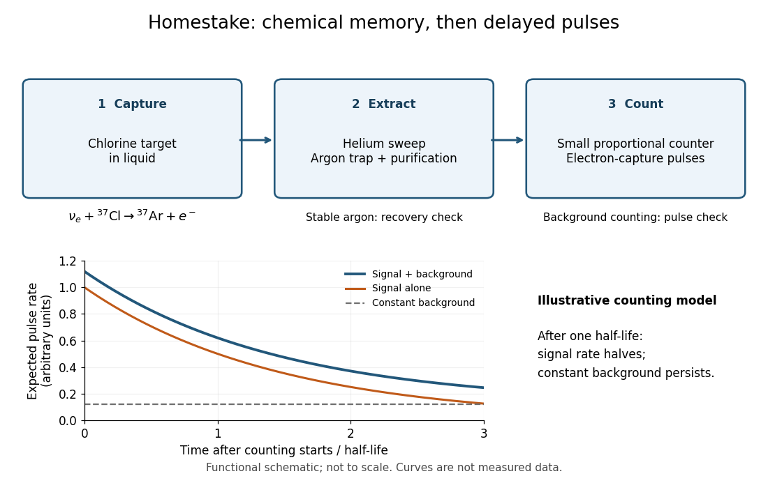
The reaction selects electron neutrinos, and its threshold excludes the lowest-energy part of the solar neutrino spectrum. A low count alone cannot distinguish a low source neutrino flux, a changed neutrino flavor mixture, or an underestimated loss in extraction or counting. This is why chemical recovery tests and an independent water Cherenkov neutrino reconstruction are scientifically valuable.

An idealized radiochemical neutrino counting model separates production, survival, recovery and readout. Suppose a freshly cleared target produces atoms at a constant rate $R$ during exposure $T$. Each atom has nuclear decay constant $\lambda =\log 2/h$, where $h$ is its half-life. The expected surviving population obeysThe proof is to multiply the differential equation by $e^{\lambda t}$ and apply integration. The expression also follows by summing the exponential decay survival probabilities of atoms produced at every earlier time. Production does not imply eventual recovery: atoms can decay during exposure.

Let $\eta$ be the fraction recovered instantaneously at extraction, $d$ the subsequent delay before counting, $ϵ$ the probability of recording a decay, and $W$ the counting duration. The expected signal pulses areWith constant background rate $b$, the expected total is $\mu ={\mu }_s+bW$. During counting, the expected instantaneous pulse rate is $s(t)+b$, with $s(t)=ϵ\eta \lambda N(T)e^{-\lambda (d+t)}$. Equal time windows therefore lose signal by the factor $e^{-\lambda \Delta t}$ while a constant background stays unchanged. Fitting the time dependence helps distinguish radioactive decay from that background; it does not recover individual capture times.

For an original worked example choose $Rh=20$, $T=W=h$, $d=0$, $\eta =0.8$, $ϵ=0.5$ and $bh=0.2$. These are illustrative assumptions. Then $N(T)=10/\log 2$, andDoubling the exposure does not double the surviving inventory: $N(2h)/N(h)=3/2$. A delay of one half-life halves the signal. At $\lambda T\ll 1$, $N(T)\simeq RT$; at long exposure it saturates at $R/\lambda$. These limits explain why a large target and repeated extraction can matter more than simply waiting longer. The model neglects time-dependent production, finite extraction duration, residual atoms between runs and time-dependent backgrounds.

The solar tachocline is the rotational transition near the base of the convection zone, approximately at $0.7$ solar radii, between differential rotation above and more nearly uniform rotation in the radiative interior. Its shear can contribute to the Omega effect, and stable stratification can help store strong toroidal magnetic fields. It is a proposed site for important parts of the solar dynamo, rather than a demonstrated unique location for all field generation.

The solar magnetic field is generated and maintained by electrically conducting flows through solar dynamo action. It includes a large-scale approximately dipolar component near activity minimum and strong, intermittent fields in active regions and sunspots. Its organized polarity reversals define the magnetic solar cycle. Magnetic stresses modify the generating flows, so a saturated dynamo requires nonlinear feedback as well as magnetic induction.

A spatially extended pattern of magnetic concentrations near boundaries of supergranulation. Surface transport and convergence redistribute magnetic elements into this network; flux emergence, cancellation and diffusion also continually modify it. It is distinct from the much smaller-scale field pattern in individual intergranular lanes and from the organized strong fields of sunspots.

The solar dynamo is the induction and regeneration of the solar magnetic field by conducting flows powered ultimately by solar convection and rotation. In a mean-field dynamo, differential rotation supplies the Omega effect and helical correlations or the Babcock-Leighton mechanism regenerate a poloidal magnetic field. The mean induction equation iswhere $\mathcal{E}=⟨\mathbf{u}\times \mathbf{b}⟩$ is the mean-field electromotive force. A model must close this correlation and include feedback to predict a saturated magnetic cycle; prescribing a shear alone does not close the regeneration loop.

Rotation influences convection, its helicity and differential rotation, which feed dynamo action. The generated magnetic field produces surface activity and strengthens the angular-momentum lever arm of a stellar wind. Wind braking lowers the rotation rate and ordinarily reduces unsaturated activity. Lorentz force feedback also changes the differential rotation and convective motions, saturating the dynamo on shorter time scales. Secular evolution, cyclic polarity reversal and irregular modulation are distinct time scales of this coupled system.

An interface solar dynamo separates the region of strong differential rotation from the region of poloidal-field regeneration, often placing shear near the tachocline and an alpha effect in the convection zone. Magnetic transport across the interface couples the two regions. The separation can provide toroidal-flux storage in a relatively stable layer, but growth, period and migration depend on the transport, diffusivity contrast, and signs of the regeneration and shear coefficients.

An ideal planar alpha-Omega dynamo places poloidal regeneration above an interface and shear-generated toroidal induction below it. With equal constant diffusivities, decay away from the interface and ordinary electromagnetic matching, its surface-wave branch grows when $D>32$ for positive $k,\alpha ,V$. The model separates the two regeneration regions while allowing diffusive coupling. The threshold refers to this model, not every solar interface dynamo or a full isotropic alpha closure.

Let $p=s-i\omega$ and $q^2=k^2+p/\eta$, with $\mathrm{Re}q>0$. The upper poloidal amplitude is $(A_0+Cz)e^{-qz}$ and the lower toroidal amplitude is $(B_0+cz)e^{qz}$. Their forcing equations give $2\eta qC=\alpha B_0$ and $-2\eta qc=ikV{A}_0$; interface matching gives $C=2q{A}_0$ and $c=-2q{B}_0$. Eliminating amplitudes yields the dispersion relation. Its potentially growing branch has $s=\eta k^2(\sqrt{D/32}-1)$ and $\omega =-\eta k^2\sqrt{D/32}$ with the convention $e^{ikx-i\omega t}$. The opposite branch decays.

For a planar interface, equal permeability and no singular sheet current make all magnetic components continuous. A nonzero horizontal Fourier wavenumber then gives the first three conditions in the title. Continuity of the tangential electric field supplies the last: continuous mean velocity cancels its advective contribution, and the retained alpha mean-field electromotive force is along the toroidal direction, so the other tangential electric component is $-U{\partial }_{x}A-\eta {\partial }_{z}B$. The given alpha-Omega equations retain only toroidal-to-poloidal alpha generation; adding a full isotropic alpha contribution would alter both the bulk equation and the matching problem.

A flux-transport solar dynamo couples toroidal and poloidal field generation through meridional advection, turbulent magnetic diffusion and possibly turbulent pumping. A common model uses the surface Babcock-Leighton mechanism, differential rotation near the tachocline, poleward surface circulation and an equatorward deep return flow. If advection dominates, circulation strongly influences the cycle period and migration; if diffusion dominates, diffusive coupling is important instead. Agreement with a butterfly pattern depends on the assumed transport geometry and coefficients, not merely on including a circulation term.

The Babcock-Leighton mechanism regenerates large-scale poloidal solar flux through the emergence and dispersal of systematically tilted bipolar active regions. With Joy's law tilt, opposite polarities have different latitudes: cancellation near the equator and poleward transport of surviving following-polarity flux alter and reverse the polar field. Thus a toroidal field that produces rising bipolar regions feeds back into a poloidal magnetic field. The source is intrinsically nonlocal between the interior flux reservoir and surface emergence and is stochastic because active-region fluxes and tilts vary.

A sunspot is a relatively cool, dark photospheric region associated with concentrated magnetic flux. The strong magnetic field inhibits convective heat transport, reducing the emergent local intensity. Spots commonly emerge in bipolar active regions, whose polarity and systematic tilt follow Hale's polarity law and Joy's law. Their number and latitude distribution are visible tracers of the solar cycle.

The axis of a bipolar solar active region is statistically tilted relative to the local east-west direction, with its following polarity typically farther from the equator and a mean tilt that grows with latitude. Scatter is substantial. The separation in latitude of the two polarities allows their surface dispersal to generate a net poloidal field through the Babcock-Leighton mechanism.

The solar cycle is the recurrent variation of magnetic activity, with a characteristic sunspot-number period of about eleven years. The large-scale magnetic polarity reverses from one activity cycle to the next, giving an approximately twenty-two-year magnetic cycle. Activity cycles vary in length and amplitude. A satisfactory solar dynamo model must account for polarity reversal, equatorward activity-belt migration in the solar butterfly diagram, the phase relation between polar and active-region fields, and long-term modulation including solar grand minima.

A solar grand minimum is a prolonged interval, lasting several ordinary cycles, of strongly reduced sunspot activity. Historical records identify the Maunder minimum; cosmogenic carbon-14 and beryllium-10 provide longer indirect records because stronger heliospheric magnetic shielding generally reduces cosmic-ray production of these isotopes. Weak activity does not imply a zero solar magnetic field. Proposed causes include stochastic weakening of poloidal-field generation, nonlinear dynamo modulation, and intermittency near an excitation threshold.

The Maunder minimum is the interval approximately 1645–1715 when recorded sunspot activity was exceptionally low. It is the best-known historical solar grand minimum. Historical coverage and cosmogenic-isotope records require care in inferring its precise magnetic amplitude; evidence for weak modulation need not imply that the normal spot-producing dynamo disappeared completely.

Bipolar solar active regions preferentially have one leading magnetic polarity in a given hemisphere and cycle, the opposite leading polarity in the other hemisphere, and reversed assignments in the next cycle. These statistical polarity rules reveal the ordered toroidal component of the solar magnetic field. Individual active regions can violate the preferred pattern, so the law is a statistical regularity rather than an exact rule for every spot pair.

A solar butterfly diagram plots sunspot occurrence or magnetic flux against latitude and time. New-cycle sunspot belts appear at middle latitudes and migrate toward the equator, producing successive wing-shaped patterns. Magnetic butterfly diagrams additionally show poleward flux transport and polar-field reversals. The diagram constrains both Parker dynamo wave propagation and magnetic transport in flux-transport solar dynamos.