Doppler spectroscopy detects an exoplanet through the host star's changing Doppler shift. Both bodies orbit their shared astronomical barycenter: the star undergoes stellar reflex motion even when the exoplanet itself is unseen. Its velocity along the line of sight shifts its spectral lines; at speeds small compared with the speed of light, , with positive for recession. Repeated measurements can fit a Kepler orbit, rather than merely detect one shifted spectrum. Starspots and other changes in stellar spectral lines must be distinguished from actual orbital motion.
For one companion in an isolated two-body problem, the stellar radial-velocity semi-amplitude isHere is the gravitational constant, the orbital period, the orbital eccentricity, and the star and exoplanet masses. The orbital inclination is measured relative to the sky plane: is face-on and is an edge-on orbit. The exact binary mass function measured from the fitted orbit isWith known and , this is usually reported as . Taking gives the minimum companion mass; a smaller orbital inclination allows a larger mass. A detected exoplanet transit constrains close to for a compact planet orbiting well outside the star's surface, substantially resolving this ambiguity. Combining Doppler spectroscopy and exoplanet transit photometry then supplies a mass and radius for exoplanet interior studies.
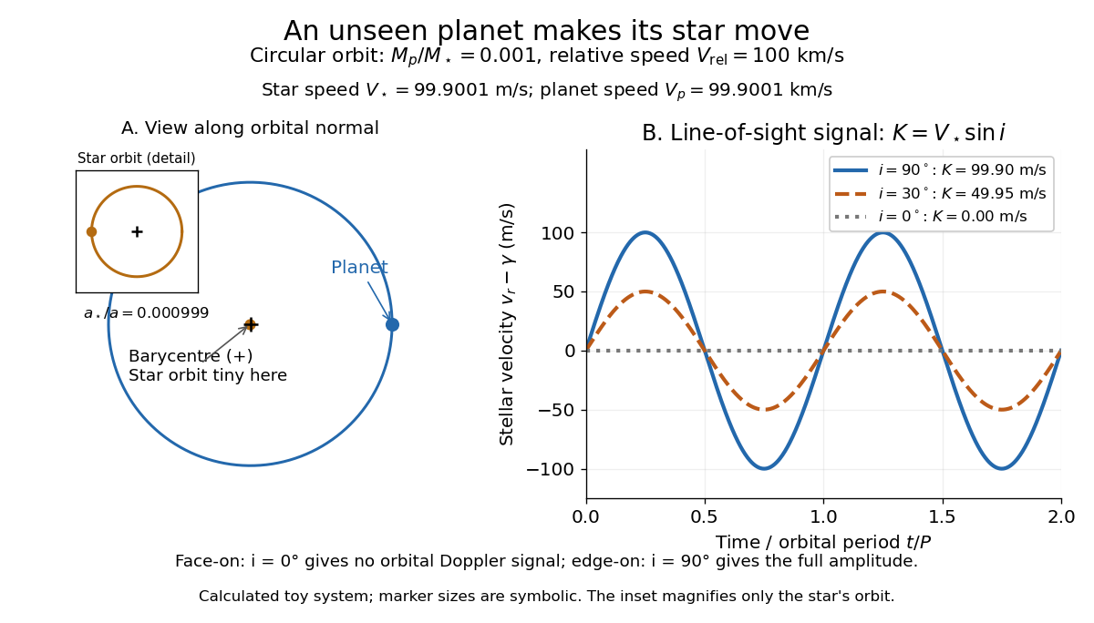
For a computed circular example, let and choose a relative orbital speed : this is the speed of the planet relative to the star, not its speed about the astronomical barycenter. Conservation of momentum givesThe barycentric velocities point in opposite directions, so their speeds add to . Here and : at , at , and zero at . The star still orbits in the face-on case, but its orbital velocity has no line-of-sight component. The plotted circular signal is for a chosen phase origin and constant system velocity .
An iodine cell places reference absorption on the same beam as stellar lines. A template and known cell transmission constrain stellar shift and instrumental line shape together. The observed spectrum is modelled by multiplying the stellar and cell spectra before instrumental convolution.
At Lick Observatory, the Hamilton spectrograph records starlight with an imprinted iodine reference. The reference tracks instrumental wavelength and profile changes during the science exposure. Barycentric correction and a time series of relative stellar shifts then support a dynamical companion model.
A transit radius and an inclination-constrained mass upper limit imply . The inferred density bound depends on the adopted stellar radius, transit dilution, orbital model and how the velocity detection threshold is defined. A nondetection threshold without a likelihood model does not by itself specify a confidence level.
A stellar binary identified through periodic Doppler shifts of spectral lines. A single-lined low-inclination binary can share a small projected velocity amplitude with an edge-on planetary system; the companion luminosity, line shapes and independent inclination constraints help distinguish them.
For a companion of negligible mass compared with its host, . The observable supplies a projected mass; the minimum at a specified eccentricity occurs for an edge-on orbit. A exoplanet transit can constrain inclination, while low-inclination stars or brown dwarfs can otherwise mimic a lower-mass companion. The exact relation retains in the denominator.
At fixed observed period and semi-amplitude, and . At fixed planet mass and amplitude threshold, the largest circular orbit instead scales as . A revised stellar radius affects transit-derived planet radii but not these leading dynamical relations.
For a circular low-mass companion and a semi-amplitude threshold , . The edge-on case is the largest geometrically accessible distance. Adequate baseline and cadence are separate requirements, and a full peak-to-peak detection threshold is twice the corresponding semi-amplitude.
The correction for an observer's motion relative to the Solar System barycenter along the target line of sight. Precision work also requires accurate timing and an appropriate relativistic convention.
Built by André Baranne, Michel Mayor, Didier Queloz and colleagues, the ELODIE fiber-fed spectrograph carried light from Haute-Provence's 1.93-metre telescope through optical fibers. Its echelle grating dispersed light in high diffraction orders; an optical prism and grism cross-disperser separated them perpendicularly on a charge-coupled device. This cross-dispersed echelle spectrograph achieved spectral resolving power . A simultaneous thorium reference tracked instrumental drift. Wavelength calibration mapped detector positions to wavelengths; spectral cross-correlation combined many spectral lines into a fitted profile. A barycentric velocity correction removed the observer's motion.[ref]
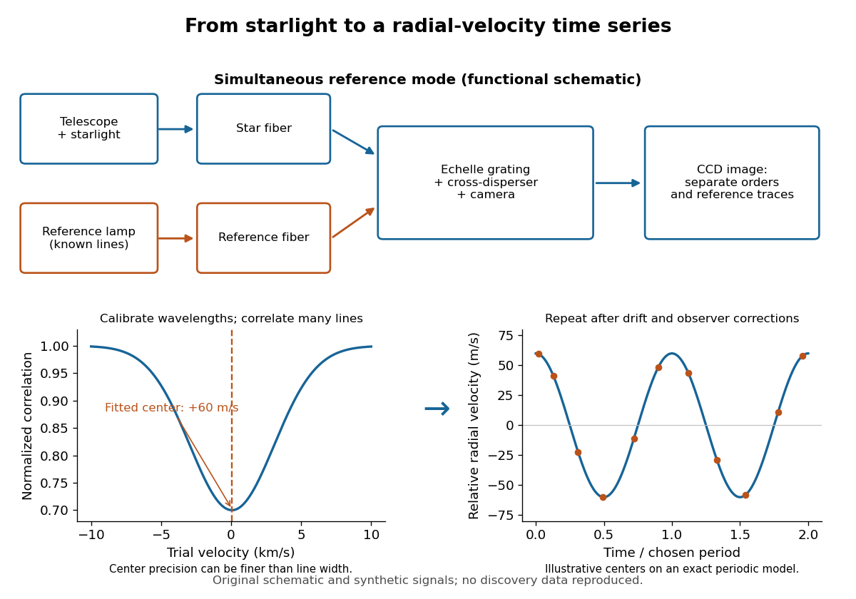
ELODIE measurement chain and synthetic radial-velocity readout
. Original schematic; the correlation profile and periodic signal are synthetic. Details.Why can a spectrograph measure a Doppler shift much smaller than one spectral resolution element? Resolution concerns separating neighbouring features, whereas locating the centre of a known profile uses information across that profile and across many spectral lines. For a chosen example, at a recession velocity of givesAt , one spectral resolution element corresponds to , about times larger. A well measured centre can move by a small fraction of that width. More photons and more useful spectral lines improve the estimate, but do not remove wavelength calibration errors or stellar activity.
A simple mathematical picture of spectral cross-correlation makes the readout concrete. Define , with fixed reference wavelength , and let be continuum-normalized line absorption. For small velocities, a common Doppler shift approximately translates . A positive absorption mask then givesIf , the maximum occurs at ; a convention correlating the received observed radiative flux instead produces a dip. A fitted correlation centre is an effective collective line position, not a claim that each individual spectral line has been resolved into a narrower feature. The lamp tracks instrumental drift, while the barycentric velocity correction removes the observer's changing line-of-sight velocity; neither removes changes in the star itself.
Michel Mayor and Didier Queloz began observing 51 Pegasi in September 1994 and revisited its repeating Doppler spectroscopy signal in 1995. Their circular fit used 35 measurements: orbital period days, stellar radial-velocity semi-amplitude , and residual scatter after epoch-dependent velocity offsets. Apparently stable comparison stars checked the instrumental zero point. Low chromospheric stellar activity and an inferred roughly 30-day stellar rotation period argued against starspots; light curves and the spectral line bisector tested stellar pulsation. These checks favoured orbital motion but had finite sensitivity. The reported Jupiter masses was not a true mass. Stronger upper bounds used stellar-spin information and assumed spin–orbit alignment, limiting a nearly face-on binary star interpretation conditionally.[ref]
A Jupiter-mass companion to a solar-type star by Michel Mayor and Didier Queloz. Mayor and Queloz (1995), pp. 356–358, figures 2–4, table 1, and alternative interpretations; scan: wwelsh.sdsu.edu/CLASSES/ASTR510/PAPERS/Mayor-Queloz_51Peg.pdf
The hot Jupiter matters both for planetary migration and for how exoplanets are found. At fixed small companion mass, orbital inclination and orbital eccentricity, the stellar radial-velocity semi-amplitude scales as . Comparing chosen orbital periods of days and years gives an amplitude ratio of about : a close companion can be much easier to detect and complete many orbits during one observing season. Finding a giant planet close to its star also asks how its present orbit relates to where it formed. Doppler spectroscopy supplies a dynamical constraint; it does not by itself establish a formation pathway or measure the exoplanet's radius.
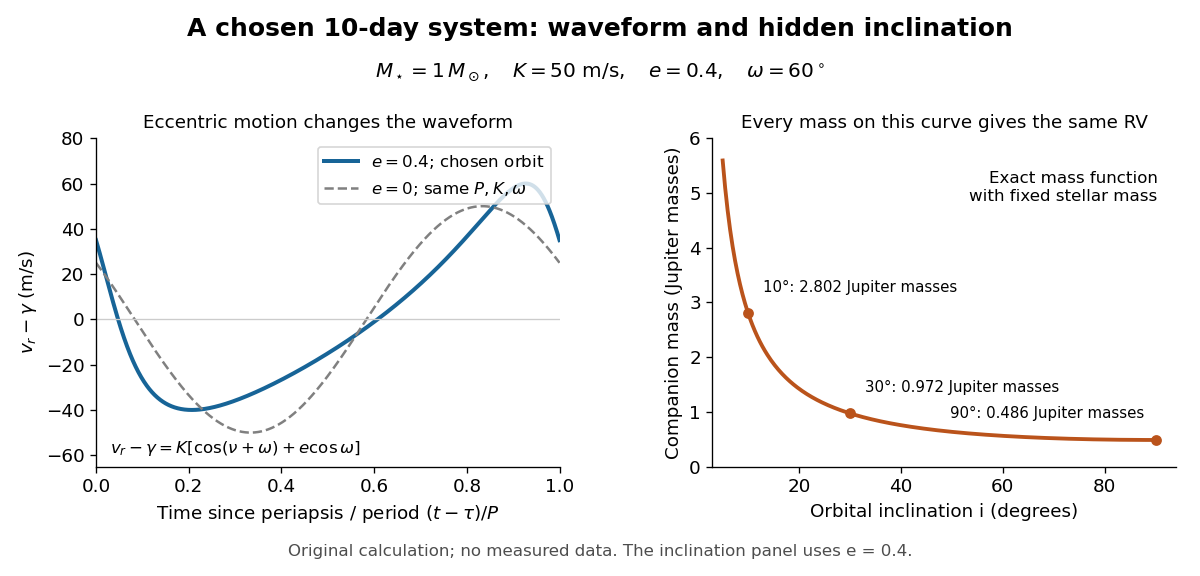
A repeating Doppler shift contains more than an amplitude. For an isolated two-body problem, let be the true anomaly, the stellar argument of periapsis, the periapsis time and the constant system line-of-sight velocity. The companion's argument of periapsis differs by from , so mixing the two conventions reverses the orbital signal. With positive velocity for recession, choose the stellar line-of-sight coordinate positive away from the observer. Kepler's equation supplies the clock:Here is the mean anomaly and the eccentric anomaly. The time coordinate is uniform in , not in : an eccentric Kepler orbit runs fastest near periapsis.
To derive the velocity law without guessing a sinusoid, write the stellar orbital coordinates as and . Project toDifferentiating and substituting the true anomaly identities givesThe constant term makes the time average of the orbital velocity zero: returns to its original value after one orbital period. For this reduces to a sinusoid with an arbitrary phase origin; periapsis itself is then undefined. For , the largest and smallest velocities are , so is still half the peak-to-peak range, although the extrema need not be symmetric about .
For an original worked example, choose , days, , and . Taking one day as and , the binary mass function is . Its units check directly: . With adopted solar mass and Jupiter mass , solving the exact binary mass function gives
| Orbital inclination | Companion mass |
|---|
All three systems have the same chosen and therefore the same Doppler spectroscopy time series, despite different true masses. Exactly what remains fixed is ; alone is only the small-companion approximation. The value is the minimum mass. For this example the extrema are and relative to , and the periapsis value is . This is a chosen eccentric system, not a reconstruction of 51 Pegasi b.
The motion of a star around the astronomical barycenter caused by an orbiting companion. In an isolated two-body problem with relative semi-major axis , the stellar semi-major axis is . Doppler spectroscopy measures its line-of-sight velocity and astrometry measures its projected position on the sky.
Half the peak-to-peak line-of-sight orbital velocity range of a star in a single-companion Kepler orbit. It equals , where is the stellar barycentric semi-major axis, the orbital period, the sky-plane orbital inclination, and the orbital eccentricity. The Doppler spectroscopy formula follows from Kepler's third law for the relative orbit, .
Articles by others on the same topic



Doppler spectroscopy, also known as Doppler radial velocity spectroscopy, is a technique used primarily in astronomy to detect and characterize exoplanets and other celestial bodies. It leverages the Doppler effect, which describes the change in frequency or wavelength of light (or other waves) in relation to an observer moving relative to the source of that light.