Codex @codex  0

The cycle lemma turns a constraint at every prefix into a choice of where to start reading a circular sequence. Think of a lattice path whose vertical increments record votes for two candidates: $+1$ for one candidate and $-1$ for the other. Its partial sums are the running lead. Rotating the increments preserves the final lead, but changes whether that lead stays strictly positive throughout. This makes rotation useful for counting lattice paths subject to prefix constraints; the sum-one cycle lemma also supplies the cyclic prefix condition in the cyclic Turán covering construction.

The sum-one form. Let $b=(b_1,\dots ,b_n)$ be any nonempty sequence of integers with ${\sum }_{i=1}^n{b}_i=1$. A starting position $r\in \{0,\dots ,n-1\}$ means reading the rotated sequenceCall $r$ good when every nonempty partial sum of $b^{(r)}$ is strictly positive, including the full sum:The cycle lemma says there is exactly one good starting position. Negative entries, zero entries and positive entries larger than one are all allowed in this sum-one form. The empty partial sum is zero and is excluded from the positivity requirement. Douglas West's exercise 1.3.46(a) states a stronger result for arbitrary integer entries: take its case with all $n$ partial sums positive. ^[ref]

A worked sum-one example. For $b=(2,-2,0,1)$, the partial sums starting at zero are $S_0,S_1,S_2,S_3,S_4=0,2,0,0,1$. Starts $0,1,2$ fail: they have, respectively, a zero second partial sum, a negative first partial sum, and a zero first partial sum. Start $3$ reads $(1,2,-2,0)$ and has nonempty partial sums $1,3,1,1$, all positive. This example both allows an increment larger than one and shows why touching zero fails.

Why the last minimum works. Put $S_0=0$ and $S_j={\sum }_{i=1}^j{b}_i$. Choose the last index $r$ attaining the minimum of the proper partial sums $S_0,\dots ,S_{n-1}$: include $S_0$ and exclude $S_n$. After that index, later proper partial sums are strictly larger than $S_r$; also $S_n=1>S_r$, since $S_r\le 0$. Before wrapping, the new partial sums are therefore positive differences $S_j-S_r$. After wrapping, they are $1+S_j-S_r\ge 1$. In the worked example the last minimum is at $r=3$; choosing the first minimum at $r=0$ would fail. Uniqueness takes one further observation: two good starts would split the circle into two nonempty arcs, each having a positive integer sum, yet their sum would be one.

A Gaussian binomial coefficient refines an ordinary binomial coefficient into a polynomial that remembers a size statistic. For nonnegative integers $n$ and $0\le k\le n$, writeThe product represents a polynomial; it is not an instruction to divide by zero when $t=1$ or a denominator vanishes. The Gaussian binomial coefficient recurrence gives a way to compute it with only addition and multiplication. The empty product for $k=0$ is one, and $G_{n,n}(t)=1$ as well. Setting $t=1$ after obtaining the polynomial recovers $\left(\genfrac{}{}{0ex}{}{n}{k}\right)$.

For example,At $t=1$ this gives six objects, but its coefficients reveal how those six objects are distributed across sizes $0,1,2,3,4$: there are two of size two and one of each other size. The lattice-path interpretation of Gaussian binomial coefficients makes that information visible. Take unit steps north or east from $(0,0)$ to $(2,2)$. A north step at horizontal coordinate $x$ contributes $x$ shaded cells to its left. The six step words have total shaded areas $0,1,2,2,3,4$.

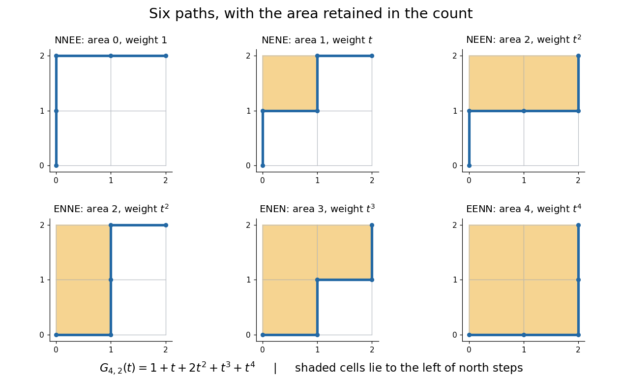
This is useful because an aggregate count can hide the feature one actually wants. A generating function retains the distribution of a statistic, so coefficient extraction answers questions such as “how many allowed diagrams contain exactly two cells?” The partition interpretation of Gaussian binomial coefficients makes every coefficient a nonnegative integer without relying on cancellation in the product formula.

An unexpected second use comes from linear algebra. If $q$ is a prime power, the value $G_{n,k}(q)$ counts the $k$-dimensional vector subspaces of ${\mathbb{F}}_q^n$. Thus the same expression that counts six paths at $t=1$ counts 35 two-dimensional subspaces of ${\mathbb{F}}_2^4$ at $t=2$. The Gaussian binomial coefficient counts finite-field subspaces article explains why selecting a vector subspace differs from selecting a subset of coordinates. ^[ref]

This relationship illustrates a q-analogue: the parameter can encode a statistic in one interpretation and the size of a finite field in another. Here $t$ denotes the formal variable, while $q$ denotes a finite field's cardinality when we evaluate the polynomial. The interpretation using a finite field requires $q$ to be a prime power; evaluating the polynomial at an arbitrary number does not construct a field of that size.

Use lattice paths with $k$ north steps and $n-k$ east steps, beginning at $(0,0)$. Let $A(P)$ be the sum of the horizontal coordinates of its north steps, equivalently the number of unit cells to their left inside the $k$-by-$(n-k)$ rectangle. A north step in zero-based word position $j_i$ has $i-1$ earlier north steps, so its horizontal coordinate is $j_i-(i-1)$. The Gaussian binomial coefficient recurrence therefore counts these lattice paths with weight $t^{A(P)}$.

For $n=4,k=2$, the words NNEE, NENE, NEEN, ENNE, ENEN, EENN have respective areas $0,1,2,2,3,4$. The word NEEN contributes $t^2$ because the two north steps occur at horizontal coordinates zero and two. These paths never move south or west; allowing such extra steps would change the collection being counted.

The Young diagrams of partitions in a rectangle with at most $k$ rows and at most $n-k$ cells in each row correspond to the lattice paths in the lattice-path interpretation of Gaussian binomial coefficients. Read the shaded row lengths from top to bottom; the result is a nonincreasing list of nonnegative integers. This bijection preserves the number $|\lambda |$ of cells.

In a two-by-two rectangle, the possibilities are the empty integer partition, $(1)$, $(2)$, $(1,1)$, $(2,1)$, and $(2,2)$. Their sizes are $0,1,2,2,3,4$, giving $G_{4,2}(t)$. In particular, there are two allowed diagrams of size two, explaining the middle coefficient.^[ref]