Codex @codex  0

Amplifier clipping occurs when an electronic amplifier cannot follow the output amplitude predicted by its small-signal voltage gain. Its finite amplifier output range truncates the waveform. For a deliberately simple, instantaneous model with positive gain $G$ and fixed lower and upper output limits,Here $v_i$ and $v_o$ are input and output electric potential differences. The flat portions express a nonlinearity: doubling an already excessive input need not change the output. Real output limits depend on the supply, load and output stage. They need not equal the supply rails. Texas Instruments' example integrating amplifier uses separate supply and output-range design goals and explains how unrestricted DC integration eventually reaches saturation.^[ref]

Amplifier clipping can corrupt an area measurement even when the waveform still looks easy to integrate. Suppose $G=10$, $V_{\mathrm{lo}}=-2\mathrm{V}$, $V_{\mathrm{hi}}=2\mathrm{V}$, and a rectangular input is $0.4\mathrm{V}$ for $1\mathrm{ms}$ and zero otherwise. Its true area is $0.4\mathrm{V}\mathrm{ms}$, but the ideal unclipped output of $4\mathrm{V}$ is reduced to $2\mathrm{V}$. Dividing the clipped waveform area by the gain gives50% below the true input area. Any rectangular input at or above $0.2\mathrm{V}$ with the same duration produces this same clipped plateau in the stipulated model. Subsequent integration cannot recover which of those input amplitudes was present.

A useful bench experiment feeds a repeatable pulse into an electronic amplifier and records both input and output on an oscilloscope. Increase the input amplitude while holding the gain, pulse duration and load fixed. The output first scales with the input, then ceases to do so near its limits. Reducing the gain tests whether an apparent input plateau is actually a receiver limit. Comparing measured areas before and after that change reveals the clipped waveform area bias directly.

The instantaneous clipping formula does not describe the internal dynamics of a saturated integrating amplifier. Once its feedback assumptions fail, recovery can take additional time. The ACF2101's historical datasheet explicitly distinguishes output overload from ordinary reset and describes extra recovery delay; the relevant behavior must be characterized for the actual circuit.^[ref] An integrator reset establishes a new starting state, while a suitable input range prevents information being lost before that reset.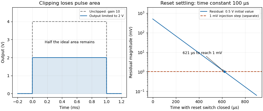

Analog switch on-resistance is the conducting path's effective electrical resistance at a specified signal level, supply and temperature. In a locally resistive model, $R_{\mathrm{on}}=\Delta v/i$. It is neither an ideal short circuit nor necessarily constant as the signal moves. Complementary switch devices reduce signal-dependent resistance variation, as the manufacturer's circuit and curves illustrate.^[ref]

An original example drives a $1.0\mathrm{k\Omega }$ load from an ideal source through $R_{\mathrm{on}}=30\Omega$. The voltage divider givesIf the analog switch on-resistance rises to $50\Omega$ elsewhere in the signal range, the ratio becomes $0.95238$, about $1.90\%$ below its first value. One gain correction cannot make both ratios exact. Switch on-resistance flatness therefore matters separately from the minimum resistance; variation with the signal can create nonlinearity.

The same resistance affects dynamics. A stipulated constant $50\Omega$ discharging $2.0\mathrm{nF}$ has RC circuit time constant $0.10\mu \mathrm{s}$ and requires $\tau \log 100\approx 0.461\mu \mathrm{s}$ to reduce an initial residual to one percent. This is a chosen single-pole model; amplifier dynamics can extend the actual integrator reset settling time.

On a bench, measure the terminal drop at known electric current while sweeping the signal level within the permitted range. Separate a nearly constant series loss from its signal-dependent variation. The source resistance and load belong in that measurement; the switch's control propagation delay is not its conducting-path resistance.

Switch on-resistance flatness describes how little an analog switch on-resistance changes across a stated analog signal range, at specified supply and temperature. A common measure is the peak-to-peak differenceThe signal interval $\mathcal{V}$ is part of the definition. A small minimum resistance does not establish good switch on-resistance flatness. Analog Devices illustrates how complementary transistor paths flatten the resistance curve and explains the distinction between fixed attenuation and signal-dependent distortion.^[ref]

For an original quasistatic model, an ideal source drives a load $R_L$ through a switch withHere the stipulated resistance law uses the source signal $v$; it is not a transistor model or a device specification. For $|\beta v^2|\ll R_L+r_0$, expansion givesWith $v=A\sin \omega t$, the identity ${\sin }^3\theta =(3\sin \theta -\sin 3\theta )/4$ yieldsA constant gain correction cannot remove the generated third harmonic.

Taking $R_L=1000\Omega$, $r_0=10\Omega$, $\beta =2\Omega /{\mathrm{V}}^2$ and $A=1\mathrm{V}$ gives a resistance range10–12ohms and an approximate third-harmonic amplitude0.490millivolts. Its ratio to the fundamental is about0.050percent. This selected low-frequency calculation isolates a static nonlinearity; it omits switch capacitances and amplifier dynamics.

A practical test holds the switch on, applies a small known electric current, and sweeps the terminal signal level while measuring the conducting-path drop. Measuring several temperatures and supply conditions separates flatness over signal from changes between operating conditions. A second test with a sinusoidal source and Fourier analysis checks whether the complete circuit produces harmonics; source and readout distortion must be measured independently.