Pareto distribution ($\mathrm{Pareto}(\alpha ,\beta )$)

The Pareto distribution describes a positive random variable whose tail probability falls as a power law. In the shape–minimum convention used here, $X\sim \mathrm{Pareto}(\alpha ,\beta )$ has shape parameter $\alpha >0$ and minimum $\beta >0$, with probability support $[\beta ,\infty )$. Its probability density function isThe minimum $\beta$ has the same units as $X$; the shape parameter $\alpha$ is dimensionless. At fixed $\alpha$, changing $\beta$ gives a scale family, since $X/\beta \sim \mathrm{Pareto}(\alpha ,1)$. This convention is also used in uniform-Pareto conjugacy.^[ref]

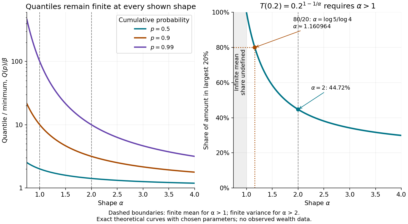
The survival function and cumulative distribution function areFor $0<p<1$, solving $F(x)=p$ gives the quantile functionIts right-hand limit at $p=0$ is $\beta$; it tends to infinity as $p\uparrow 1$.^[ref] There is no probability mass at $\beta$: changing a probability density function's value at that single point changes no probabilities.

Choose $\alpha =2$ and $\beta =10$ as an original theoretical example. Then $\mathbb{P}(X>20)=1/4$, $\mathbb{P}(X>100)=1/100$, the median is $10\sqrt{2}\simeq 14.142$, and the 0.99 quantile is $Q(0.99)=100$. These chosen values and all figures below describe mathematical probability distributions, not actual wealth observations.

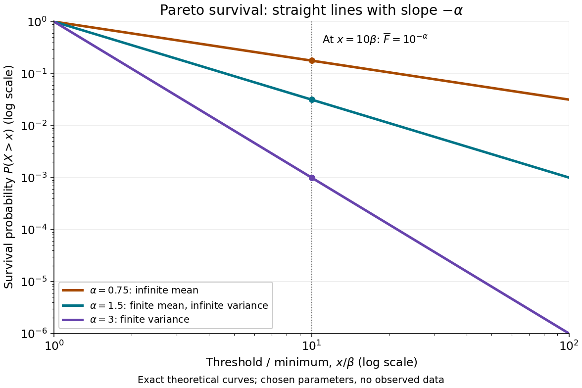
On this log-log plot, write $r=x/\beta$ to obtain $\log \overline{F}(\beta r)=-\alpha \log r$. The slope is $-\alpha$, whereas the probability density function has power exponent $\alpha +1$. Multiplying a threshold by ten divides its tail probability by $10^{\alpha }$. A larger $\alpha$ therefore concentrates the Pareto distribution nearer $\beta$; a smaller $\alpha$ makes extreme values more plausible. This exact scaling is useful when modelling large positive losses or sizes over several orders of magnitude.

The Pareto distribution is a heavy-tailed distribution: for every $t>0$, the exponential moment $\mathbb{E}[e^{tX}]$ diverges because $e^{tx}{x}^{-\alpha -1}$ eventually grows without bound. In contrast, the Laplace distribution has exponentially decreasing tails and some finite positive exponential moments. The Student's t-distribution also has power tails, but on both sides of the real line, with a smooth central region rather than a positive minimum.

Let $X$ have survival function $\mathbb{P}(X\ge x)=x^{-s}$ for $x\ge 1$, with $s>1$. Its expected value is $s/(s-1)$. The tail-sum formula for expectation givesThe absolutely continuous probability distribution gives zero mass to the integers, so $\lceil X\rceil =\lfloor X\rfloor +1$ almost surely and $\mathbb{E}[\lceil X\rceil ]=\zeta (s)+1$. Taking expectations of $\lfloor X\rfloor \le X\le \lceil X\rceil$ gives $\zeta (s)\le s/(s-1)\le \zeta (s)+1$, which rearranges to the displayed bounds on the Riemann zeta function. Finiteness is justified by $\lfloor X\rfloor \le X$ and $\lceil X\rceil \le X+1$.

For the Pareto distribution of shape $a>0$ and lower bound $b>0$, the density $a{b}^a{x}^{-a-1}$ is strictly decreasing on $[b,\infty )$. Its highest-density interval of probability $1-\alpha$, $0<\alpha <1$, must begin at $b$. The tail probability $\mathbb{P}(X>u)=(b/u{)}^a$ makes the upper endpoint $u=b{\alpha }^{-1/a}$. If this is a posterior distribution, the result is its highest posterior density interval. In particular, Uniform-Pareto conjugacy supplies posterior shape $a+n$ and lower bound $\max (b,{\max }_i{y}_i)$.

Let $S_n={\sum }_{i=1}^n{X}_i$, where the summands are independent and identically distributed with Pareto distribution $\mathrm{Pareto}(\alpha ,\beta )$. Their positivity implies $\{X_1\ge na\}\subseteq \{S_n\ge na\}$, so for fixed $a>0$ and $na\ge \beta$,Both outer expressions tend to zero. A single large summand already prevents a strictly negative exponential rate. No positive exponential moment exists, so the exponential-moment form of the Cramér theorem cannot be applied. The bound proves this logarithmic rate and does not assert an exact tail asymptotic. In particular, it remains true when $a$ lies below a finite mean, where the event need not even be rare. The stronger fixed-summand-count asymptotic in a heavy-tailed subexponential distribution is a separate statement.

A Pareto distribution is a proper probability distribution for every $\alpha ,\beta >0$, even when its mean is infinite. To see both facts, integrate the probability density function against $x^q$. For real $q\ge 0$,The improper integral converges exactly when $q-\alpha -1<-1$. At $q=\alpha$ it diverges logarithmically; above that it diverges as a positive power of the upper endpoint. Setting $q=0$ gives one, proving normalization regardless of whether higher moments exist.

Taking $q=1,2$ and using $\mathrm{Var}(X)=\mathbb{E}[X^2]-(\mathbb{E}[X]{)}^2$ when both terms are finite givesFor $0<\alpha \le 1$, the nonnegative random variable has expected value $+\infty$; a centered variance about a finite mean is unavailable. For $1<\alpha \le 2$, the mean is finite and the variance is infinite.^[ref] A finite total probability and a finite expected value answer different questions.

At the chosen minimum $\beta =10$, $\alpha =3$ gives $\mathbb{E}[X]=15$, $\mathbb{E}[X^2]=300$ and variance $300-15^2=75$, but an infinite third moment. At $\alpha =3/2$, the mean is 30 and the variance is infinite; at $\alpha =3/4$, even the mean is infinite, while the median remains the finite number $102^{4/3}\simeq 25.198$. At the boundary $\alpha =2$, the earlier example has mean 20 but infinite variance. A finite sample contains finite values almost surely; that fact cannot establish that the underlying mean or variance is finite.

Conditioning a Pareto distribution on exceeding a threshold changes its minimum while preserving its shape parameter. For $u\ge \beta$ and $x\ge u$, the definition of conditional probability givesEquivalently, for $r\ge 1$,The ratio to the threshold has the same Pareto distribution at every admissible threshold.^[ref] For the chosen $\alpha =2$, $\beta =10$, only $1/4$ of outcomes exceed 20, but among those outcomes the probability of exceeding 40 is again $1/4$. When $\alpha >1$, the same identity gives conditional expectation $\mathbb{E}[X\mid X\ge u]=\alpha u/(\alpha -1)$.

This multiplicative scaling differs from the additive memoryless property of an exponential distribution. Indeed $Y=\log (X/\beta )$ has exponential distribution of rate $\alpha$, because $\mathbb{P}(Y>y)=e^{-\alpha y}$ for $y\ge 0$. Thus logarithms turn multiplication into addition and explain the scaling property. Conversely, if $U$ has uniform distribution on $(0,1)$, inverse transform sampling gives $X=\beta (1-U{)}^{-1/\alpha }$.

The excess $Z=X-u$ conditional on $X\ge u$ has survival function $(1+z/u{)}^{-\alpha }$ for $z\ge 0$. In the generalized Pareto distribution convention $\mathbb{P}(Z>z)=(1+\xi z/\sigma {)}^{-1/\xi }$, this means $\xi =1/\alpha$ and $\sigma =u/\alpha$. Here the excess starts at zero; the original Pareto distribution starts at $\beta >0$.

For a nonnegative random variable with finite positive mean, the share of its total amount carried by the largest fraction $q$ of outcomes can be defined by dividing their contribution to the expected value by the whole expected value. For a Pareto distribution, let $0<q\le 1$ and choose $x_q=\beta q^{-1/\alpha }$, so that $\mathbb{P}(X\ge x_q)=q$. If $\alpha >1$, direct integration givesThis is a share of amount, distinct from the fraction of outcomes. It depends on $\alpha$, but not on the unit of measurement $\beta$.^[ref]

For the chosen $\alpha =2$, the top 20% starts at $x_{0.2}=10\sqrt{5}\simeq 22.361$ and carries $T(0.2)=\sqrt{0.2}\simeq 44.72\%$ of the amount. To make the top 20% carry exactly 80%, solveThe resulting Pareto distribution has a finite mean and infinite variance. The 80/20 rule selects one shape parameter; it is not a universal law, or even a property of every Pareto distribution. For $\alpha \le 1$, the population-share definition above is unavailable because its denominator is infinite; substituting such an $\alpha$ into the finite-mean formula is invalid.

The left panel compares three quantiles in units of the minimum. The right panel shows $T(0.2)$ only where the mean is finite, and marks the chosen 80/20 value. The thresholds $\alpha =1$ and $\alpha =2$ separate the moment regimes; they do not separate valid and invalid probability distributions.

A straight-looking empirical log-log plot does not by itself establish a Pareto distribution or a reliable tail exponent; estimating an exponent and assessing goodness of fit are separate tasks.^[ref] If a Pareto distribution is used only above a fitted lower threshold, $T(q)$ describes that conditional tail population, not automatically the whole population. A genuine finite upper cutoff gives a truncated distribution with finite nonnegative moments; its survival function, quantiles and top shares must be recalculated. Truncation is a modelling change, distinct from merely observing a finite sample. None of the chosen numbers here estimates an actual wealth distribution.