Past exam of the algebra 1 and differential equations 1 course of the University of Oxford / 2015 / 4 / b

Factor each component of the vector field. The horizontal-velocity nullclines and vertical-velocity nullclines are, respectively,The last curve is a hyperbola. In the nonnegative quadrant its branch is $y=2/x$ for $x>0$.

Intersect the two nullcline families. The axes yield $(0,0)$ and $(1,0)$, and $y=1$ with $xy=2$ yields $(2,1)$. The possible remaining intersection would have $x+y=1$ and $xy=2$, requiring $x^2-x+2=0$, whose discriminant is $-7$. Hence there are no further real equilibria.

The Jacobian matrix isEvaluate it at each equilibrium:

All three are hyperbolic equilibria, so their classifications persist for the nonlinear system. Immediately to the right of $(2,1)$ on $y=1$, the velocity is vertically downward, showing that the attracting spiral turns clockwise.

For $x,y>0$, the signs needed for the phase portrait follow directly from the factorizations:The coordinate axes are invariant sets. On $y=0$, the logistic differential equation $\dot{x}=x(1-x)$ directs positive states toward the boundary saddle point $(1,0)$. On $x=0$, $\dot{y}=2y$ directs positive states upward. At the three equilibria, use the local directions found in part (ii); interior sample trajectories near $(2,1)$ spiral clockwise inward.

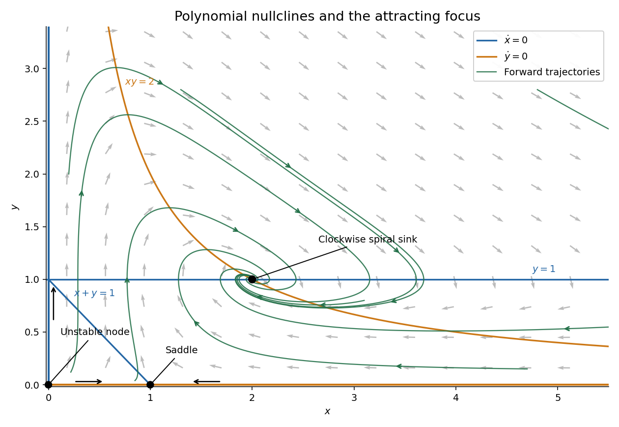
The nullclines prescribe where arrows become vertical or horizontal; they are generally not themselves trajectories. The image samples the vector field and several solutions, rather than assuming every nullcline is an invariant set.