Algebra 1 and differential equations 1 course of the University of Oxford (A1)

Historical Part A paper title printed on the 2015 examination.

Source release: Oxford examination archive, member FOI-20210708-1 - Data/a13753w1.pdf. The cover dates this examination to 17 June 2015, 9.30am–12.30pm.

All six questions and their 38 leaf subparts are answered below. The unnumbered criterion at the start of 2(a) has its own solution before the four field cases.

The identity $T^2=T$ gives the decompositionThe first summand lies in the kernel of a linear map $\ker T$, and the second in the image of a linear map $\mathrm{im}T$. If $w$ belongs to their intersection, write $w=Tu$; then $Tw=T^{2}u=Tu=w$, while $Tw=0$. Thus $w=0$, proving the direct sumOn these two invariant subspaces, $T$ is respectively zero and the identity map. Joining a basis of each produces a basis of eigenvectors, with matrixHence every linear projection is diagonalizable, over the original field, including in characteristic two.

Put $n=\dim V>0$ and $r=\mathrm{rank}T$. The direct sum in part (i) givesThe eigenvalues are the members of $\{0,1\}$ actually present: zero occurs exactly when $r<n$, and one exactly when $r>0$. Since $T$ is diagonalizable, its minimal polynomial contains each present eigenvalue once:In particular, a nonzero vector space does not force both eigenvalues to occur. The zero and identity maps are important special cases.

The same invariant subspaces work for $S=\alpha I+\beta T$: it acts by $\alpha$ on $\ker T$ and by $\alpha +\beta$ on $\mathrm{im}T$. Its minimal polynomial is therefore the product of the distinct linear polynomials belonging to the nonzero summands. Explicitly,When $\beta \ne 0$, the two candidate eigenvalues are distinct in any field. This is the minimal polynomial of an affine function of a projection.

Expand the square using $E^2=E$ and $F^2=F$:ThusThis sum of two linear projections criterion holds in every characteristic; it uses an equality of linear maps, not cancellation of factors in the noncommutative associative algebra of linear endomorphisms.

Suppose first that $E+F$ is a linear projection. Part (i) gives $EF=-FE$. Multiplying on the left by $E$ gives $EF=-EFE$, and multiplying on the right by $E$ gives $EFE=-FE=EF$. Combining them yieldsIn a field of characteristic different from two, the nonzero scalar $2$ is invertible. Hence $EF=0$, and $FE=-EF=0$ too. Conversely these two zero products make the expansion in part (i) equal zero. ThereforeThe argument cancels a nonzero scalar, never a possibly singular linear map.

No. On any nonzero vector space over a field of characteristic two, take $E=F=I$. Both are linear projections, andThe correct condition from part (i) in this characteristic is $EF=FE$, because minus and plus coincide. Vanishing of both products remains sufficient, but is no longer necessary.

The proposed equivalence is false. On a nonzero vector space over any field of characteristic different from two, chooseThese linear projections commute and satisfy $EFG=0$. Nevertheless their sum is $2I$, andThus the proposed conditions are not sufficient. For commuting linear projections the actual obstruction is the sum of the pairwise products:The single condition on the triple product does not remove this obstruction.

A linear endomorphism is diagonalizable over its field precisely when its minimal polynomial is a product of distinct linear polynomials over that same field. Splitting alone is insufficient: repeated factors permit nontrivial Jordan blocks.

For the displayed matrix, a determinant expansion givesThese formulas can be reduced in each requested characteristic. The four cases below distinguish failure to split from failure to have distinct factors.

Over the complex numbers, the three eigenvalues areThey are distinct. Each is a root of the minimal polynomial, so here the minimal polynomial equals the characteristic polynomial and has distinct linear polynomials. Consequently $A$ is diagonalizable over $\mathbb{C}$.

The quadratic polynomial $x^2+4x+10=(x+2{)}^2+6$ has no real roots of a polynomial. Thus the characteristic polynomial does not split over the real numbers. A real diagonal matrix would have only real eigenvalues, and similar matrices have the same characteristic polynomial. Therefore $A$ is not diagonalizable over $\mathbb{R}$.

In the finite field ${\mathbb{F}}_3$, reduce the characteristic polynomial to $(x-1{)}^3$. For $B=A-I$, reduction of the entries givesHenceIts repeated linear polynomial prevents diagonalizability. Equivalently, a diagonalizable map with only the eigenvalue one would have to be $I$, and this matrix is not $I$.

In the finite field ${\mathbb{F}}_2$, the matrix becomesOn the first two coordinate vectors it is a nonzero nilpotent Jordan block of size two, and on the last it is the identity map. ConsequentlyThe repeated zero root prevents diagonalizability. Directly, the only possible eigenvalues are zero and one, so diagonalizability would imply $A^2=A$, whereas the displayed off-diagonal entry disappears on squaring.

The primary decomposition theorem for linear maps states that ifwith distinct monic irreducible polynomials $p_j$, thenEach summand is a $T$-invariant subspace. More generally the same direct sum conclusion holds for any factorization of an annihilating polynomial into pairwise coprime polynomials, using the corresponding kernels. The underlying mechanism is the Bézout's identity for polynomials, which separates the mutually coprime factors.

Since $T$ is diagonalizable, its minimal polynomial is ${\prod }_{j=1}^r(x-{\lambda }_j)$ with distinct eigenvalues ${\lambda }_j$ in the field. Apply the primary decomposition theorem for linear maps:For a scalar that is not an eigenvalue, the associated eigenspace is zero, so the sum indexed by the whole field has only finitely many nonzero summands. The eigenspaces need not be one-dimensional.

For $v\in V_{\lambda }$, use commutation to obtainThus $Sv\in V_{\lambda }$, proving that every $T$-eigenspace is an $S$-invariant subspace. This does not assert that an arbitrary eigenvector of $T$ is already an eigenvector of $S$.

On each nonzero eigenspace $V_{\lambda }$, the restricted linear map $S_{\lambda }=S{|}_{V_{\lambda }}$ is diagonalizable. Indeed $m_S(S_{\lambda })=0$, so the minimal polynomial of $S_{\lambda }$ divides $m_S$. A divisor of a product of distinct linear polynomials has the same property, proving the diagonalizable restriction lemma.

Choose a basis of $S_{\lambda }$-eigenvectors in each $V_{\lambda }$. Every chosen vector is simultaneously a $T$-eigenvector, with eigenvalue $\lambda$. The direct sum in part (ii) shows that joining these bases gives a basis of $V$. Therefore $S$ and $T$ have a common eigenbasis, which is exactly simultaneous diagonalization.

Suppose a single basis gives the diagonal matrices $D_S,D_T$. Entrywise multiplication gives $D_S{D}_T=D_T{D}_S$. If $P$ is the change-of-basis matrix, thenThus simultaneous diagonalization implies commutation.

Yes, provided “commute” means pairwise commute. Necessity follows because three diagonal matrices commute pairwise.

For sufficiency, first choose the common eigenbasis for the first two linear maps, say $S,T$, obtained in part (b). Their joint eigenspacesgive a direct sum decomposition of $V$. The third map $U$ preserves each $W_{\lambda ,\mu }$, since $SUv=USv=\lambda Uv$ and $TUv=UTv=\mu Uv$. By the diagonalizable restriction lemma, $U{|}_{W_{\lambda ,\mu }}$ has a basis of eigenvectors there. Every such vector already has fixed eigenvalues for $S$ and $T$.

Joining these bases therefore gives a common eigenbasis for all three maps. The same induction proves simultaneous diagonalization for any finite pairwise commuting family of diagonalizable linear endomorphisms.

The dual basis is the collection of linear functionals characterized byExplicitly, $e_i^{\prime }({\sum }_j{\alpha }_j{e}_j)={\alpha }_i$. Every linear functional $\ell \in V^{\prime }$ satisfies $\ell ={\sum }_i\ell (e_i)e_i^{\prime }$, proving that the displayed functionals span the dual space. Evaluating a zero linear combination at each $e_j$ makes all its coefficients zero, so they are also linearly independent. Thus they form a basis of $V^{\prime }$.

Define the bidual evaluation map by evaluation:For fixed $v$, this is a linear functional of $\ell$, so it belongs to the double dual. It is also linear as a function of $v$. If $v\ne 0$, some coordinate of $v$ in a basis is nonzero, and the corresponding dual basis functional detects it. Hence $J(v)\ne 0$, proving injectivity.

The spaces $V,V^{\prime },V^{\prime \prime }$ all have the same finite dimension. Therefore an injective linear map $J:V\to V^{\prime \prime }$ is surjective, proving the required linear isomorphism.

This linear isomorphism is natural because evaluation requires no basis. More explicitly, for any linear map $A:V\to W$, its dual map satisfiesso $A^{\prime \prime }{J}_V=J_{W}A$.

Writing $u={\sum }_i{u}_i{e}_i$ and $v={\sum }_i{v}_i{e}_i$, evaluation against the dual basis givesThis has codomain $\mathbb{C}$, not the printed $\mathbb{R}$. For a nonzero vector space, take $u=i{e}_1$ and $v=e_1$ to obtain $\varphi (u,v)=i$. Only the diagonal values $\varphi (v,v)$ must be real. The displayed formula defines the intended complex inner product.

It is linear in the first argument and conjugate-linear in the second:It has conjugate symmetry, since $\varphi (v,u)=\overline{\varphi (u,v)}$. Finally,with equality exactly when every coordinate vanishes, equivalently $v=0$. This proves positive definiteness. Since $\varphi (e_i,e_j)={\delta }_{ij}$, the original basis is orthonormal. This is the inner product determined by a basis.

Use the convention of part (a): the inner product is linear in its first argument. If $Tv=\lambda v$ with $v\ne 0$, the adjoint operator identity and $T^{\ast }=-T$ givePositive definiteness makes $⟨v,v⟩>0$, soThus every eigenvalue of a skew-adjoint operator is purely imaginary, including zero.

Take $v\in U^{\perp }$ and $u\in U$. Because $U$ is an invariant subspace, $Tu\in U$. The adjoint operator relation yieldsThis holds for every $u\in U$, so $Tv\in U^{\perp }$. Therefore the orthogonal complement is also an invariant subspace.

Proceed by induction on the dimension. For positive dimension, the fundamental theorem of algebra gives a root of the characteristic polynomial, hence a nonzero eigenvector $v$. Normalize it to have norm one. Its span is an invariant subspace, and part (ii) makes its orthogonal complement invariant too:The restriction of $T$ to the complement remains skew-adjoint, since the same inner product identity holds there. The induction hypothesis supplies an orthonormal eigenbasis for that smaller space. Adjoining $v$ gives an orthonormal eigenbasis for $V$.

The zero-dimensional base case is immediate. Thus $T$ is diagonalizable, indeed unitarily diagonalizable. This proves the finite-dimensional case of the spectral theorem for a skew-adjoint operator without assuming that distinct eigenvalues have multiplicity one.

Regard the real skew-symmetric matrix as acting on ${\mathbb{C}}^n$. Its Hermitian adjoint is $A^{\ast }=A^T=-A$. Parts (i) and (iii) show that its eigenvalues are purely imaginary and its complex minimal polynomial has no repeated roots.

Since $A$ has real entries, nonreal eigenvalues occur in conjugate pairs. A nonzero pair has the form $i\alpha ,-i\alpha$, with $\alpha >0$, and contributes the real quadratic polynomialZero, if present, contributes one factor $x$. Hence the real minimal polynomial isThe product annihilates $A$ after complexification of a real vector space, so it also annihilates the original real linear map; no factor can be removed because each displayed complex root is an eigenvalue. This proves both the asserted form and its minimality. The case $A=0$ has $\epsilon =1$ and an empty product.

An autonomous differential equation has no explicit dependence on the independent time variable: its vector field depends only on the current state. The two families of nullclines areOn the first family the horizontal velocity is zero; on the second the vertical velocity is zero. A critical point of a dynamical system is a state where both components vanish. It gives a constant solution, also called an equilibrium.

Translate the equilibrium to the origin by $z=(x-a,y-b{)}^T$. If the vector field is continuously differentiable, its first-order Taylor expansion isThe Jacobian matrix $M$ gives the linearization $\dot{z}=Mz$, whose general solution is $z(t)=e^{tM}z(0)$ using the matrix exponential. Its eigenvalues determine the exponential factors, while its eigenvectors and, when necessary, generalized eigenvectors determine their directions.

For distinct eigenvalues ${\lambda }_1,{\lambda }_2$ and corresponding eigenvectors $v_1,v_2$,For a real matrix with nonreal conjugate eigenvalues, choose conjugate coefficients to obtain real solutions. Equivalently, if $\lambda =a+ib$ and $v=p+iq$, a real pair of independent solutions isFor a repeated eigenvalue $\lambda$, there are two cases:

The factor $t$ in the second case is essential. These are exact solutions of the linearization; the remainder describes the error for the nonlinear differential equation. When no eigenvalue has zero real part, the hyperbolic equilibrium theory justifies the corresponding local qualitative classification. Zero real parts require additional nonlinear analysis.

Factor each component of the vector field. The horizontal-velocity nullclines and vertical-velocity nullclines are, respectively,The last curve is a hyperbola. In the nonnegative quadrant its branch is $y=2/x$ for $x>0$.

Intersect the two nullcline families. The axes yield $(0,0)$ and $(1,0)$, and $y=1$ with $xy=2$ yields $(2,1)$. The possible remaining intersection would have $x+y=1$ and $xy=2$, requiring $x^2-x+2=0$, whose discriminant is $-7$. Hence there are no further real equilibria.

The Jacobian matrix isEvaluate it at each equilibrium:

All three are hyperbolic equilibria, so their classifications persist for the nonlinear system. Immediately to the right of $(2,1)$ on $y=1$, the velocity is vertically downward, showing that the attracting spiral turns clockwise.

For $x,y>0$, the signs needed for the phase portrait follow directly from the factorizations:The coordinate axes are invariant sets. On $y=0$, the logistic differential equation $\dot{x}=x(1-x)$ directs positive states toward the boundary saddle point $(1,0)$. On $x=0$, $\dot{y}=2y$ directs positive states upward. At the three equilibria, use the local directions found in part (ii); interior sample trajectories near $(2,1)$ spiral clockwise inward.

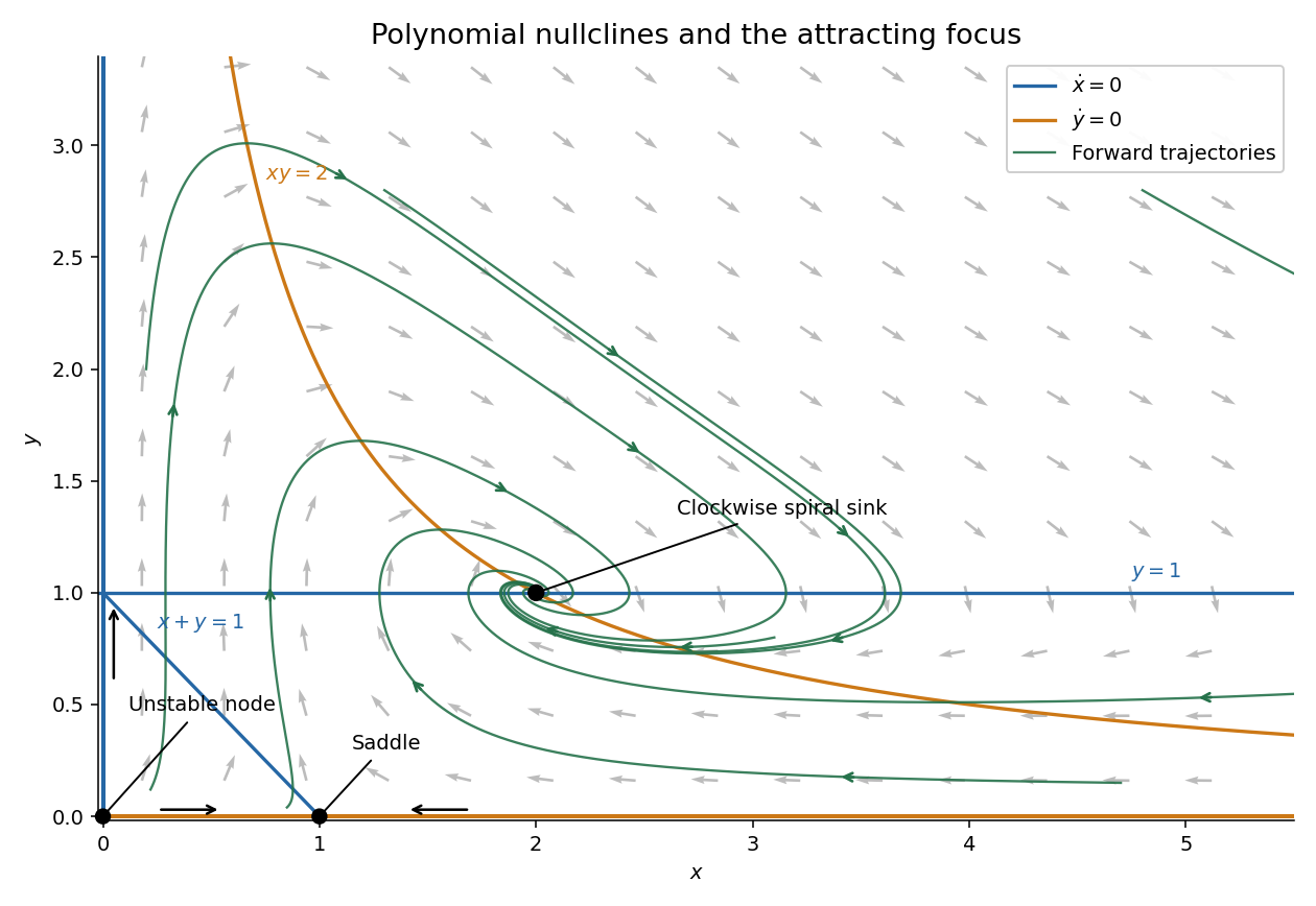
The nullclines prescribe where arrows become vertical or horizontal; they are generally not themselves trajectories. The image samples the vector field and several solutions, rather than assuming every nullcline is an invariant set.

For a second-order linear partial differential equation written $A{u}_{xx}+2B{u}_{xy}+C{u}_{yy}+\cdots =0$, the discriminant is $B^2-AC$. HereIt is positive exactly when $x\ne 0$, proving that the equation is a hyperbolic partial differential equation on each half-plane. At $x=0$ its principal part degenerates and it is not hyperbolic.

The characteristic curves satisfyIntegrating suggests the characteristic coordinatesTheir Jacobian determinant is $2/x$, so this is an invertible local change of variables whenever $x\ne 0$. Write $u(x,y)=U(\xi ,\eta )$. The chain rule givesSubstitution cancels both unmixed second derivatives and both first derivatives:The canonical form of a second-order partial differential equation is thereforeThe cancellation of the first derivatives is the key feature of these logarithmic characteristic coordinates.

Integrate the canonical form of a second-order partial differential equation first in $\eta$ and then in $\xi$. The first integration gives $U_{\xi }=\eta +g^{\prime }(\xi )$, and the second givesThusThe two arbitrary twice continuously differentiable functions describe the two characteristic families. Conversely, substituting this expression into $U_{\xi \eta }=1$ verifies every such solution. The formula applies on $x>0$ or $x<0$; independent choices can be made on the two half-planes. Smooth extension across the degenerate line $x=0$ requires extra compatibility and is not supplied by the logarithmic formula alone.

Use the classical regularity setting $u\in C^2(D)\cap C(\overline{D})$, with $D$ bounded. Continuity on the compact set $\overline{D}$ guarantees existence of a minimum. The inequality $\Delta u=f\le 0$ means that $u$ is superharmonic function.

A strict inequality $\Delta u<0$ would immediately exclude an interior minimum, because its Hessian matrix there would be positive semidefinite and have nonnegative trace. To handle equality, introduce the quadratic perturbation proof of the minimum principle:Its minimum must lie on $\partial D$. Choose $R$ so that $x^2+y^2\le R^2$ on $\overline{D}$. For any $p\in D$,Letting $\epsilon \downarrow 0$ gives $u(p)\ge {\min }_{\partial D}u$. ThereforeThis asserts that a minimum is attained on the boundary, not that it cannot also be attained inside; a constant function attains it everywhere.

For a harmonic function, $\Delta u=0$ and $\Delta (-u)=0$. Apply the preceding minimum argument to $u$ and to $-u$:These are the weak minimum and maximum principle for harmonic functions.

The difference $w=v-u$ is a harmonic function, because the Laplacian is a linear differential operator:The boundary inequality says $w\ge 0$ on $\partial D$. The minimum principle from part (ii) givesThis is the comparison principle for harmonic functions. Applying it in both directions also shows why fixed Dirichlet boundary conditions determine at most one harmonic function.

Introduce the position and velocity variables $y_1=y$ and $y_2=y^{\prime }$. Then the required system of ordinary differential equations and initial condition areThus $f_1(x,\mathbf{y})=y_2$. Conversely, the first equation identifies $y_2=y_1^{\prime }$, and the second recovers the original second-order ordinary differential equation and both initial data.

Work with the L1 norm on ${\mathbb{R}}^2$. The scalar Lipschitz hypothesis impliesWe may take $L\ge 0$. The compact set $S$ and continuity give a finite bound $M={\max }_S\Vert \mathbf{f}{\Vert }_1$. ChooseLet $I=[a-\eta ,a+\eta ]$. The space $C_{\eta }$ of continuous maps $I\to B_k(\mathbf{b})$ is complete in the supremum norm: it is a closed subset of the Banach space $C(I,{\mathbb{R}}^2)$. Define the Picard operator on a closed ball byFor any $\mathbf{g}\in C_{\eta }$, the integral triangle inequality givesThe integrand is continuous, so the result is continuous and remains in the prescribed closed ball. Thus $\mathcal{P}$ is a self-map of the complete space. Moreover,It is a contraction mapping. The contraction mapping theorem gives a unique fixed point $\mathbf{y}$. By the fundamental theorem of calculus, the fixed-point identity makes $\mathbf{y}$ continuously differentiable and gives ${\mathbf{y}}^{\prime }=\mathbf{f}(x,\mathbf{y})$ and $\mathbf{y}(a)=\mathbf{b}$. Its first component is twice continuously differentiable, because its derivative is the second component.

Conversely, integrating any solution that remains in the ball makes it a fixed point, so it equals $\mathbf{y}$. A solution starting at $\mathbf{b}$ cannot first reach the boundary of this ball during $I$: before such an exit the same estimate gives distance at most $\eta M<k$, contradicting distance $k$ at the first exit. This proves existence and uniqueness on $|x-a|\le \eta$, not merely formal convergence of an iteration. It is the local Picard-Lindelöf theorem construction.

In position-velocity variables $(u,v)$, the scalar right-hand side isIts only relevant singularity is $u=0$. The initial state $(x,u,v)=(0,1,1)$ is separated from it. For an explicit application of part (a), take $h=1$ and $k=1/2$ in the L1 norm. On the resulting closed ball, $1/2\le u,v\le 3/2$, and $|x|\le 1$.