For a steady spherical, nonrotating, bounded collisionless galaxy, the mean velocity vanishes, the mixed velocity moments vanish, and . A steady radial stellar flux would satisfy ; regularity and no central source/sink set that constant to zero in the equilibrium model. The Spherical Jeans equation is thereforeHere is the tracer number density, not necessarily the gravitating mass density. Random motions supply the velocity stress balancing the gravitational field.
Two conventions in the printed general equation need correction before interpreting it outside this special limit. Its first standalone derivative of mean radial velocity should be a time derivative, , not : the latter has incorrect acceleration dimensions. Also a velocity dispersion is the centered moment . The printed raw-moment definition equals it only when the mean velocities vanish, as they do in the equilibrium used here. These issues do not change the simplified result above.
For an ensemble of nearly circular stellar orbits with randomly oriented planes, radial motion is small while tangential motion is substantial: . The two tangential variances remain equal by spherical symmetry. There need not be bulk rotation even though individual stars move on nearly circular paths. The anisotropy parameter is strongly negative; its exactly circular limit is singular as .
Nearly radial orbits have small transverse motion: . A bounded steady population contains both inward and outward phases, so large radial dispersion is compatible with zero mean radial velocity. Positivity of the distribution function and stability can impose further restrictions on particular radial models.
An isotropic velocity distribution has equal variance in every direction and zero mixed moments:This is a statement about random velocity directions at each radius, not a requirement that every star follows a circular orbit.
For spherical gravity, . Inserting into the Spherical Jeans equation and solving for the total enclosed mass givesThe mass includes all sources of the potential, including dark matter or a central compact object; the stellar tracer density need not follow total mass. The bracket must yield nonnegative enclosed mass in a physically admissible model. Density, radial stress and anisotropy are independent observational/model inputs before this equation becomes a mass estimate.
TODO: the original line-of-sight geometry figure on source page 8 is unavailable. The PDF calls an unembedded image and the documented archive parent has the same gap. Its exact drawn layout cannot be checked or reproduced. The surviving coordinate definitions suffice for the following standard spherical-projection derivation; no missing plotted values or drawn dimensions are supplied here.
The spherical density projection schematic below is original geometry constructed from these definitions, not a recovered examination figure.
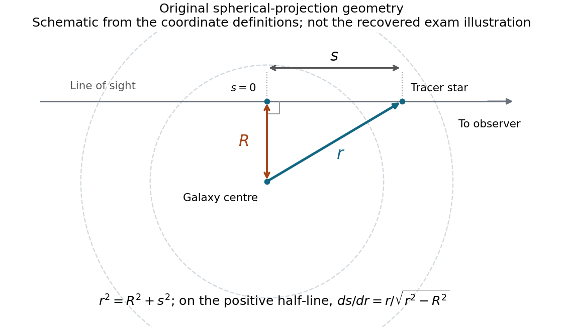
Original line-of-sight geometry from the surviving coordinate definitions; not the recovered examination figure
. Details. 
Let be closest approach on a line of sight at projected radius . Euclidean spherical geometry gives . On either half-line, , and the two halves contribute equally. With identical stellar luminosity , , soFor an isotropic velocity distribution, the variance of any unit-direction projection equals . Explicitly, the line-of-sight contributions have weights from the radial component and from a tangential component; equality of their variances makes the sum . ConsequentlyWithout isotropy the integrand instead has the factor . Thus the projection assumption is substantive, rather than something that can be inferred from spherical surface brightness alone. The missing illustration does not prevent recovering these algebraic expressions from the prose.
For the isotropic Jeans-Abel mass inversion, let and . The two preceding projections have the same Abel integral equation kernel, givingTheir ratio recovers , and the isotropic Jeans equation givesEquivalently put and . Then : the common stellar luminosity cancels from the inferred mass. Differentiating these singular-kernel integrals is understood through suitable regularity or a nonsingular variable change, not by naively keeping an infinite lower-end boundary term.
The inversion assumes adequate radial coverage, convergence and a smooth spherical equilibrium. In practice derivatives amplify noise and the unobserved outer tail needs treatment or a model. Unknown anisotropy reintroduces a mass–anisotropy degeneracy; the uniqueness just derived is conditional on the explicitly isotropic velocity distribution.
Articles by others on the same topic
There are currently no matching articles.