Source bundle pages 18–24. The cover establishes 2022 despite the attachment's 2021 filename. Solutions use SI units unless stated otherwise.
The specific intensity is energy transported per unit time, projected area, solid angle and frequency. The path coordinate increases along the ray. The emission coefficient is emitted energy per unit time, volume, solid angle and frequency, whereas the absorption coefficient has units of inverse length. Thus adds specific intensity and removes it. Stimulated emission can be included as negative absorption.
Define the optical depth between two points by . Multiplying the radiative transfer equation by the integrating factor and integrating givesEach local contribution is attenuated only by the material between its emission point and the observer. Where , the source function is and the same formal solution of the radiative transfer equation is . A constant source function gives .
Use the Einstein coefficients convention in which multiplies spectral radiation energy density , with . A normalized spectral line profile obeys . The spontaneous emission probability per upper-state atom per unit time is ; the stimulated emission and upward absorption rates per atom are respectively and .
For isotropic spontaneous emission, transitions occur per unit volume and time, each supplying photon energy . Dividing among steradians givesFor a small incident beam, its contribution to is . Absorption removes and stimulated emission adds photons in the incident direction. Matching the net loss to therefore givesReplacing by across the narrow spectral line profile gives the printed expressions. The negative sign is essential: an inverted population can amplify the incident specific intensity. Thermal equilibrium and the Planck function imply and , where is the state degeneracy. A convention using mean intensity instead changes both coefficients by .
With the spontaneous emission term suppressed, . A uniform absorption coefficient over length gives directlyThe normalized specific intensity deficit is unchanged by conversion between wavelength and frequency, since both numerator and denominator acquire the same Jacobian determinant. The Boltzmann distribution and the Einstein coefficients give . Consequently, in the optically thin limit,Here is the column density, and has been used in slowly varying factors. This linear relation between equivalent width and column density fails once the central optical depth becomes appreciable.
For the unresolved Lyman-alpha line, the lower and combined upper state degeneracies are and , so the Einstein coefficients giveThe measured equivalent width then impliesAssume a central transverse line of sight through a uniform filament, so . Nearly all neutral hydrogen is in its ground state at this temperature, henceThe cylinder's length determines its total volume but does not enter a transverse column density. Geometry must be specified: an axial line of sight has and gives for the same measured equivalent width. Intermediate chords give intermediate path-dependent estimates. The numbers above treat as a rest-frame equivalent width; an observed value at redshift must first be divided by .
True thermal equilibrium requires a thermal ionizing radiation field as well as chemical balance; equality of photoionization and recombination rates alone would require a specified external radiation field. Under the stronger equilibrium assumption, apply the Saha equation to pure hydrogen. The electron spin factor cancels the ground-state electronic degeneracy, givingAt , and . Charge neutrality gives . Importantly, the known quantity from d is the neutral number density, not the total number density; use Saha neutral fraction from a measured neutral density to obtain . ThereforeThis extraordinarily small neutral fraction is the result of applying thermal equilibrium to dilute intergalactic gas; it is not a realistic inference from photoionization equilibrium with a nonthermal cosmic background. For the axial geometry of d, the equilibrium neutral fraction is smaller by .
Adopt the stipulated neutral fraction , independently of the equilibrium estimate in e. For pure hydrogen, . The thermal Sunyaev-Zeldovich effect measures integrated electron pressure:Using the same absorbing line of sight as in d,Thus one such filament is below the stated measurement sensitivity. If the number density inferred transversely is instead used to view the same cylinder end-on, its path is twenty times longer and , still below the stated sensitivity. Changing the assumed path of the original absorption measurement while keeping its column density fixed does not change its predicted . The quoted neutral-fraction floor is a premise of this estimate, not a universal bound derivable from thermal equilibrium.
There are two different physical interpretations. The supplied logarithmic integral signals free fall in a fixed singular isothermal sphere, with a test particle moving through a frozen background. Write . By the shell theorem, the enclosed mass is and the radial equation of motion isThe second equality follows by multiplying by and using the initial rest condition. The free fall trajectory is given implicitly byThus the intended fixed-profile answer isA collapsing material shell gives a different answer. If the entire cloud undergoes pressureless gravitational collapse from rest, the edge follows the fixed enclosed mass , not the instantaneous fixed-profile value . With no shell crossing, , soThis is a concrete counterexample to treating the fixed-profile result as the exact collapse time of the whole nebula. The initial mean density inside is , consistent with the usual free-fall time of a uniform sphere expressed using that mean density. The logarithmic integral is valid for the explicitly frozen background approximation.
Assume an isolated, bound, nonrotating Newtonian gas cloud, negligible surface pressure, negligible magnetic and radiation stresses, no persistent bulk flow, and a stationary or time-averaged virialized state. The stellar virial theorem then reduces towhere is the total gravitational potential energy. Define the volume-averaged pressure and average gravitational energy density . HenceEquivalently, for a nonrelativistic monatomic gas, the thermal internal energy obeys . This second derivation must not count the thermal motions again as a separate bulk kinetic energy. If the external pressure is , the correct result is ; non-negligible bulk motion adds to the virial theorem. The initial sharp-edged profile need not survive virialization; maintaining that profile hydrostatically to its edge would generally require a surface term.
For a family of spherical profiles with a fixed dimensionless shape, write the gravitational potential energy as , where depends on that shape. The virial theorem in b and the sphere volume giveFor a uniform density, ; formally integrating for gives . Neither the virial theorem nor the initial profile guarantees a specific final shape, so the proportionality requires the stated homologous-profile assumption. Surface pressure must be handled consistently with b before using either coefficient as an equilibrium model.
For a regular spherical star, let and . The stellar mass conservation equation and stellar hydrostatic equation areAssuming the smoothness needed for the requested Taylor series, write . There is no point mass at the centre, so , and matching the stellar mass conservation equation gives , . Substitution in the stellar hydrostatic equation gives , henceThe remainder orders use a smooth spherically symmetric scalar density, for which . Merely finite continuous density gives the same leading coefficients with and remainders. In particular , despite the apparent in the stellar hydrostatic equation.
For a gas-pressure-supported stellar core of fixed mass and composition, neglect boundary terms for the illustrative whole-core estimate. The virial theorem gives , and the monatomic gas gives . Thus the effective heat capacity along the equilibrium sequence isThis negative heat capacity of a virialized gravitational system means that net energy loss makes a self-gravitating core contract and heat. It is different from the positive local material specific heat capacity. On the main sequence, hydrogen burning supplies most of the radiated energy, so rapid contraction is arrested. Hydrogen depletion increases the mean molecular weight; slow structural readjustment usually raises the central temperature rather than making it fall.
After core hydrogen exhaustion, a massive stellar core contracts and heats more rapidly until a later nuclear fuel ignites. There is no general reversal to cooling simply upon leaving the main sequence. If radiation pressure becomes dominant, the internal energy becomes with . The virial theorem therefore gives ; the radiation-dominated limit is marginally bound and its effective adiabatic index approaches .
Quasistatic contraction can still maintain virial equilibrium. It fails dynamically only when sufficient support is lost, for example if pair creation reduces the effective adiabatic index below , or when an iron core undergoes electron capture and photodisintegration. A fixed-composition gas-dominated contracting core with is already a counterexample to any assertion that leaving the main sequence alone reverses the heating or destroys virial equilibrium.
Primordial density contrasts perturb the intrinsic photon temperature, the gravitational potential, and the velocity of the last-scattering material. Intrinsic photon-density fluctuations obey because ; adiabatic initial conditions relate these to matter density contrasts. Subsequent acoustic evolution, Doppler effect and gravitational frequency shifts determine the observed Cosmic microwave background anisotropy. There is no scale-independent identification of the final sky map with matter density contrast alone.
The spherical harmonic coefficients are random variables inherited from these perturbations. After subtracting the mean sky temperature, for the anisotropy modes. Gaussian primordial perturbations give approximately Gaussian random variables; this extra Gaussian assumption is not needed for diagonal covariance. Reality of the sky map implies .
For a statistically isotropic sky, its two-point function depends only on . Rotations mix the components at fixed and do not mix different irreducible spaces. A rotation-invariant covariance matrix is therefore a multiple of the identity in each block:On our one sky, average the angular components at fixed , or equivalently suitable rotated sky pairs, rather than treating different universes as observed samples. The CMB angular power spectrum is estimated byUnder the Gaussian, full-sky, noiseless assumptions, there are independent real degrees of freedom and . This cosmic variance remains even with perfect detectors; a finite sky mask and detector noise add further uncertainty. The estimator is unbiased, , but does not turn one realization into the exact ensemble mean.
Insert the diagonal covariance from a into the two-point function and apply the spherical harmonic addition theorem:The Legendre polynomials encode the angular separation. Since , the zero-separation value is the total variance. For measured Cosmic microwave background anisotropy, remove the monopole and usually the kinematic dipole, so the corresponding sum starts at ; an instrument's angular response supplies an additional window function.
The ordinary Sachs-Wolfe effect combines intrinsic last-scattering temperature with the gravitational redshift of photons escaping the last-scattering gravitational potential. For adiabatic large-scale perturbations in matter domination, with the potential convention in the question, the combination is , up to the observer monopole. It is distinct from the Integrated Sachs-Wolfe effect caused by a time-varying potential along the later line of sight.
Use the Fourier transform convention in which is the matter power spectrum and . The Poisson equation becomes , givingWith the matter-dominated critical-density approximation ,independent of . Thus the Harrison-Zeldovich spectrum gives scale-invariant potential fluctuations and the requested dependence. Keeping a general present matter fraction would insert ; the answer here follows the stipulated critical matter-dominated normalization. In this Fourier transform convention, has dimensions of length to the fourth power.
The finite angular resolution of COBE DMR suppresses small angular scales, so only low spherical harmonic multipoles can be recovered usefully. The approximate relation associates with scales of order ten degrees; this is an effective sensitivity and beam-window limit, not a mathematical hard truncation.
Interpret the printed superscript uncertainty as . Its square estimates the band-limited zero-separation variance, rather than the full :Use the coefficient supplied in the paper for this numerical inference. With ,so c givesThe stated amplitude uncertainty gives approximately relative uncertainty in , or , keeping fixed. The ideal matter-era Sachs-Wolfe plateau with precisely the c spectrum convention has coefficient , rather than ; the supplied numerical coefficient is about larger and has been treated as the paper's prescribed approximation. A real beam-convolved analysis retains its window function and additional cosmological transfer effects.
An ultrarelativistic electron has kinetic energy much larger than its rest energy: , equivalently . Its speed obeys and its total energy is approximately . At , .
Diffusive shock acceleration is viable in principle at : repeated scattering off magnetic irregularities on opposite sides of a strong nonrelativistic shock wave can reach such energies. Actual viability requires a sufficiently large and long-lived accelerator with an acceleration time shorter than its escape and loss times; alone does not establish those conditions.
Take positive velocity toward the upstream material, and let the front move at in the upstream rest frame. For a strong adiabatic shock wave in a gas with adiabatic index , the Rankine-Hugoniot conditions give and the shock-frame inflow speeds satisfy , . The signed velocities in the three frames areThus the two scattering media converge at . For a crossing particle with incident energy in its local plasma rest frame, a Lorentz transformation to the approaching other plasma giveswhere is the incident direction cosine measured toward the approaching medium and . For an almost isotropic crossing population, flux weighting gives . Scattering randomizes directions without changing energy in that plasma frame, and the reverse crossing has the same mean gain. ThereforeThese are first-order mean gains. They are not an increase of energy in one fixed frame caused by an instantaneous boundary crossing. Literally choosing the electron's instantaneous rest frame gives incident , and the other gas approaches at nearly , so the expansion in small is invalid. This concrete frame check explains why the printed description of must instead refer to the upstream/downstream scattering frames.
The magnetic Lorentz force is perpendicular to velocity, so it does no work and remains constant over an orbit when radiative losses are neglected. For the transverse momentum, and . HenceSince ,This is the gyromotion frequency, not the much higher characteristic synchrotron radiation frequency.
Relativistic beaming concentrates the emission into a forward cone about the instantaneous velocity. The aberration of light maps a rest-frame ray at to , so the characteristic cone half-angle is . Thus its conventional full width is .
The isotropic-emission assumption has no beam nulls. For example, its received bolometric angular power is proportional to , where the Doppler factor is . In particular it is nonzero at , disproving a literal null there. A true dipole pattern for an accelerated electron is not isotropic in its rest frame and needs a specified polarization and viewing plane. The width just quoted is a characteristic beaming angle, not a null-to-null width under the stated premise.
For a circular orbit seen in its orbital plane, let the velocity direction sweep past the observer through . The emission interval is . The observed interval must also include light-travel compression:Its ratio to the gyromotion period is . Since the boundary of a smooth beam is conventional, only the scale is invariant under reasonable pulse-width definitions. For helical motion the viewing geometry and pitch angle are additional inputs; the numerical estimate assumes transverse motion and a sightline intercepted by the cone.[ref]
Essential Radio Astronomy by James J. Condon and Scott M. Ransom. Chapter 5, section 5.1.3: relativistic beaming and the difference between emission duration and pulse arrival duration
One explanation is an upper electron energy imposed by the accelerator: finite age, finite confinement size, escape, or a balance of acceleration and losses limits to . Since the synchrotron critical frequency scales as , the absence of higher-energy electrons produces a corresponding high-frequency cutoff, broadened by the single-particle spectrum.
The other is synchrotron cooling, with inverse Compton scattering often contributing: gives . High-energy electrons disappear fastest, so a population of age develops a cooling scale and . A burst population can develop a strong cutoff. With continuous power-law injection, the simplest steady cooling model instead steepens the electron energy index by one and the synchrotron radiation spectral index by , giving a break rather than necessarily an exponential cutoff. The detailed spectral shape therefore distinguishes finite acceleration from aging and injection history.
Let and . Assume the one-particle distribution function and its weighted tails decay enough that all required velocity integrals converge and boundary terms at infinite velocity vanish. Multiply the steady Collisionless Boltzmann equation by and integrate over velocity. In Cartesian coordinates, spatial differentiation commutes with this integration, while integration by parts givesConsequently the three force-balance equations areExplicitly the component is , with cyclic counterparts for . For equal stellar masses, multiplying by the common mass replaces by the mass density ; for multiple stellar masses, use a mass-weighted one-particle distribution function or derive a separate equation for each tracer population.
Define mean streaming velocity and the velocity dispersion tensor . The zeroth velocity moment of the steady Collisionless Boltzmann equation gives the continuity equation . ThereforeSubstituting in a yields the standard steady Jeans equations:The unsteady version adds on the left. Defining the stellar pressure tensor makes the analogy with fluid momentum balance explicit. The off-diagonal terms are correlations between random velocity components; they need not vanish or equal the diagonal terms.
The Jeans equations express local momentum conservation for a collisionless stellar system, just as the Euler equations do for a gas. The mean streaming velocity plays the role of fluid flow, the gravitational force is a body force, and random stellar motions supply a pressure tensor through . Taking moments smooths over individual stellar orbits and produces fields of density, mean velocity and random-motion stress; this is the sense of “stellar hydrodynamics”.
Ordinary gas pressure is usually nearly isotropic because collisions relax its local velocity distribution. A collisionless stellar system can retain an anisotropic velocity ellipsoid, so its pressure tensor is not generally a scalar times the identity. There are more unknown second moments than momentum equations, and their evolution introduces higher moments. The Jeans equations therefore require further dynamical assumptions or a specified one-particle distribution function for closure; they do not by themselves establish local thermal equilibrium or a gas equation of state.
Use fixed masses in an isolated Newtonian -body system, with origin at its centre of mass. Define the moment and . Twice differentiating givesInsert the gravitational equation of motion and pair each ordered term with :Thus one component of the tensor virial theorem isA stationary or time-averaged bounded system has , yielding . If ordered and random motions are separated, , where and . Summing the three diagonal equations recovers the scalar virial theorem, with the pair gravitational potential energy counted once.
Treat the long-wavelength nearly uniform spherical perturbation as a separate locally homogeneous expanding region, neglecting pressure gradients and tidal corrections. Its local Friedmann equation isThe curvature term represents the spatial curvature of an FLRW universe in the local patch; for the convention dimensionless, has units of inverse time squared. Positive corresponds to a closed, more tightly bound patch. Here and below the printed is interpreted as mass density or energy density divided by ; literal SI energy density requires on the right.
The region generally has its own scale factor and Hubble parameter. The two printed equations with an identical can be compared as a leading-order equal-expansion construction: on a slicing where , use in the already first-order curvature term to obtain . This equal-expansion curvature overdensity construction does not make them both exact evolution equations with a permanently identical expansion history at common proper time. For example, a growing dust density contrast obeys the continuity equation , which is nonzero when . This explicit example prevents an inconsistent identification of the two local histories.
Within the equal-expansion construction of a, subtract the flat-background Friedmann equation to obtainThe background density scales as during radiation domination and during matter domination. ThereforeThese are the regular adiabatic growing-mode scalings on scales outside the Hubble radius, with a specified time slicing. In a consistent comoving description the numerical relation between curvature and density contrast differs from the naive subtraction, but the powers agree. The result does not imply that every gauge's density contrast, every decaying mode, or subhorizon dark matter during radiation domination has these powers.
For , a regular adiabatic perturbation follows the large-scale density contrast growth in b; this does not require causal communication across the perturbation. Since , the Friedmann equation gives during radiation domination and during matter domination. A fixed comoving perturbation has physical size , so its ratio to decreases as or until cosmological horizon entry.
The numerical “exactly at equality” assertion is inconsistent with the supplied parameters and . Normalize and use the supplied as the whole radiation component. ThenBoth terms must be retained at matter-radiation equality. The present comoving size corresponding to its Hubble radius isIts physical size then is . A mode with has physical size only at equality, already inside the Hubble radius. More explicitly, putting in givesThis is a direct numerical counterexample using the stated data. Neglecting one component exactly at equality instead gives , which also does not produce . Late-time dark energy is negligible at these early times.
For conserved nonrelativistic dark matter and radiation, and , so obeys . Denote differentiation with respect to by a prime. ThenThe supplied Friedmann equations implySubstitution in the linear growth equation and division by give the Mészáros equationFor , and , making the two remaining terms cancel exactly. For reduction of order, put and . The equation reduces to , whenceUsing the supplied antiderivative and reversing an irrelevant overall sign gives the independent solutionIts Wronskian is . The asymptotic expansions areThus subhorizon dark matter during radiation domination has constant and logarithmic modes, rather than the superhorizon growth of b. A combination with negative supplies positive logarithmic growth. During matter domination, the growing mode is proportional to , agreeing with b, while the second mode decays as . These results neglect subhorizon radiation clustering; the Mészáros equation is the approximation stated in the question, not a full photon–matter perturbation system through horizon entry.
For a mode, evolve the regular superhorizon density contrast as until cosmological horizon entry. In the radiation domination approximation its entry scale is , well before matter-radiation equality. At that point use the Mészáros equation basis of d, fixing both constants by continuity of and , equivalently and .
Explicitly, for entry data and , solveThe nonzero Wronskian guarantees a unique match. This produces slow logarithmic growth before equality, then with a decaying transient after equality. For example, at , and . An abrupt match estimates the growth history; a precise amplitude requires a common gauge and the coupled relativistic perturbation equations through entry. Linear evolution also ceases to apply once approaches unity, and late dark energy further suppresses growth.
The cover identifies the 2021 examination; the source bundle's filename uses 2020. This paper occupies bundle pages 21–27. TODO: recover the damaged source plots for question 5(a)–(c). The solutions below distinguish results derivable from the surviving material from measurements that require an intact figure. Units are SI unless specified.
A hydrogen recombination line is a discrete spectral line produced when radiative recombination captures an electron into an excited bound level and a subsequent radiative cascade emits photons. The free-to-bound capture itself produces a continuum; the later bound-to-bound transitions produce the recombination lines. For example, H-alpha is the transition in the Balmer series.
For the neutral hydrogen absorbing an ionizing stellar continuum, the principal bound-free transition is photoionization from the ground state into the continuum. Most neutral hydrogen is in its ground state, and the photoionization cross section is largest near its threshold, falling approximately as above it. Dominance of the population-weighted opacity is intended here; this does not mean that every excited-state microscopic cross section is smaller at every frequency.
In an ionization-bounded, optically thick nebula, direct radiative recombination into emits an ionizing photon that promptly photoionizes another hydrogen atom. One ion disappears and another is created: there is no net removal of an ion from the global budget. Case B recombination therefore uses , with local recycling of ground-state recombination photons. This is the on-the-spot approximation, rather than an unconditional property of radiative recombination: if those photons escape, direct capture does produce net neutralization and a Case A treatment is appropriate.
Write for the hydrogen-ionizing photon production rate, counting only photons above the hydrogen ionization energy, not all stellar photons. In steady photoionization equilibrium, the external supply balances the volume integral of net Case B recombination:For uniform, almost completely ionized pure hydrogen, . HenceThe final approximation requires . The Strömgren sphere also assumes spherical symmetry, a sharp ionization front, a steady source older than the recombination time, uniform number density and temperature so that is constant, negligible dust absorption of ionizing photons, negligible leakage, and no important helium correction or collisional ionization. Clumping would replace by a volume average of .
An additional atomic input is needed: the total Case B recombination coefficient does not specify the number of H-alpha photons per net radiative recombination. Let , where is the effective recombination coefficient. At the approximately temperature implicit in the supplied , take . The coefficient 2.2 used later in the paper corresponds to , which we use consistently here.
For an unextinguished, fully filled Strömgren sphere with negligible central cavity, the H-alpha luminosity and observed radiative flux satisfySubstitution eliminates and givesConvert the angular diameter to radians: . Also . ThusThe implied hydrogen-ionizing photon production rate is . Using instead gives . These values use the printed milliarcseconds and integrated line observed radiative flux. Assuming one H-alpha photon per recombination would give a different, unjustified distance. An appreciable cavity or a nonunit filling factor must also enter the emitting volume.
The Brackett series consists of transitions ending at , at infrared wavelengths. They suffer much less interstellar extinction than H-alpha, so their corrected observed radiative fluxes can give a more reliable version of the same inference. At fixed measured angular size and number density, the formula has : uncorrected interstellar extinction therefore makes this particular distance estimate too small. Infrared lines are weaker and need their own effective recombination coefficients; their advantage is reduced sensitivity to dust.
Let be the photoionization rate per neutral hydrogen atom just outside the empty cavity. With an isotropic central source and no attenuation inside that cavity,The cross section is zero below threshold; this permits the lower integration limit zero. Pure hydrogen with hydrogen ionization fraction has and . Local photoionization equilibrium is thereforeDefine the dimensionless quantity . Solving the resulting quadratic equation, , gives the physical rootThe rationalized form avoids numerical cancellation for small . Strong illumination gives ; weak illumination gives .
Eliminating with the H-alpha luminosity, , yieldsThe printed definition of is inconsistent with the defined radii. The source calls a physical stellar radius, but its factor gives units of length to the fourth power, rather than a dimensionless value. It also omits the physically necessary cavity radius . For a concrete counterexample, double while holding the source, , and fixed: the incident photoionization rate falls by four, so rises by four; the printed expression does not change. The root has the requested form with the corrected above. There is no supplied relation allowing to be replaced by .
Retain the consistent of d. Across a sufficiently thin layer, the neutral hydrogen column density is . The direct stellar continuum acquires optical depth . Define the photon-weighted second momentExpanding the attenuating exponential in the photoionization rate givesThe second cross section moment appears because the radiation both undergoes absorption and is weighted by the photoionization cross section in computing the rate.
In a local plane-parallel approximation that suppresses geometrical dilution, setThen local photoionization equilibrium becomes , soThis gives the requested algebraic dependence, with the corrected definition of . Besides , linear attenuation requires over the frequencies contributing appreciably to the rate. In particular must remain positive.
The source's neglects , which is also first order in layer thickness. A consistent spherical first-order answer uses in the same root. Neglecting dilution relative to absorption additionally requires . As a concrete limiting test, with negligible absorption the source's predicts no change, while inverse-square dilution still decreases and thus .
Take the initially expanding branch ; the printed squared velocity alone also permits an initially contracting branch, which would not reach a future maximum radius. Multiply the equation of motion by and integrate. The conserved outer-shell specific orbital energy isThe initial mass follows from the background critical density:ConsequentlyIf means the energy of a test shell of mass , . If it means the total energy of the entire uniform, homologously moving perturbation, direct integration instead gives , andThe common convention of writing the first integral as is therefore an energy per unit shell mass, not the total energy of the sphere.
At spherical-collapse turnaround, , so . HenceAny positive initial density contrast binds this pressureless perturbation in the stated Einstein-de Sitter universe.
For and , differentiation givesComparison with proves . Substitution into the conserved specific orbital energy gives . ThereforeThese constants exactly reproduce both the initial radius and expanding velocity. The initial parameter obeysIn an Einstein-de Sitter universe whose background big bang is , . Thus the exact required offset isExpanding givesOne cannot set exactly at finite while retaining the stated initial Hubble velocity and background time origin. For example , gives . Shifting to removes the offset from the local orbit, but the background then scales as , not . Setting is justified in the early-initial-time limit for subsequent evolution; the following standard growing-mode formulae use that approximation.
First retain the exact initial normalization. The scale factor obeys , so the cosmological redshift isAlso and . Using givesThese equations exactly accommodate the finite-time initial conditions in b.
Now neglect and retain leading order in . Since , the cosmological redshift relation reduces toDefine . ThenThe second equality is exact for the ideal common-bang growing-mode spherical-collapse model; it is approximate for the paper's finite-time initial Hubble-velocity data.
The factor has a physical origin. Linear mass conservation gives when the initial local expansion equals the background Hubble flow. The general linear dust solution is . Imposing and yieldsThus is the present extrapolation of the growing component, after neglecting the decaying transient. It is not the exact present value of the full linear solution for finite .
In the growing-mode spherical-collapse model, use and . Their ratio in c gives . Meanwhile , and the linear growing density contrast scales as . Matching at small therefore fixesThis is a linearly extrapolated growing-mode amplitude at any epoch, including epochs where the actual density contrast is nonlinear. It carries the initial-condition qualification in c.
Numerical comparison isThe last column measures the fractional underestimate of the actual density contrast. Linear theory is accurate at , but substantially underpredicts it by the time approaches unity. At , the shell reaches spherical-collapse turnaround; .
At , and the ideal pressureless density diverges at finite time . Yet the extrapolated linear value remains finite:This is the linear spherical-collapse threshold, not the true density contrast at collapse. Actual nonspherical collisionless systems undergo shell crossing and virialization rather than becoming uniform point singularities. The ideal virial theorem and conservation of energy estimate a final radius if the structural form is preserved.
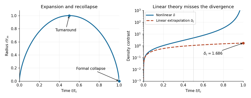
Parametric spherical collapse and the failure of the extrapolated linear density contrast
. Details. 
Work in the source rest frame and neglect the source's small cosmological redshift. Over an emission interval , a ballistic relativistic jet feature travels , advancing toward the observer and across the sky. The second photon has a shorter journey, so its arrival is delayed by onlyDividing the projected displacement by this arrival interval givesApparent superluminal motion is a combination of projection and light-travel delay. The feature's local speed remains ; its inferred transverse displacement divided by the observer's arrival interval is not a local signal velocity.
For fixed , differentiate the apparent speed with respect to angle:The maximum lies at and has value . Hence strict apparent superluminal motion requiresThe threshold is an infimum: equality yields exactly at , rather than a strictly superluminal value. For a chosen larger , the optimal inclination is , and the full superluminal interval satisfies .
For intrinsically symmetric oppositely directed relativistic jets, their proper motions areThe ratio removes and yieldsTaking the product instead givesCausality requires , so the limiting distance and inclination areHere and in e, “maximum” denotes the limiting bound; massive ejecta obey strict inequalities. The conversion is , henceBoth bounds occur together in the light-speed limit. At any specified smaller distance, determines the intrinsic speed.
The Doppler factors for the two discrete blobs are . Their ratio is . Lorentz-invariant specific intensity means is unchanged; with and the same rest-frame power-law spectrum,The brightness ratio at the common observed frequency therefore givesThe stated identical intrinsic specific intensities must refer to comparable intrinsic states. If the blobs fade with their proper ages, equal observer times sample different ages and need that correction. A steady continuous jet has a different boosting exponent, ; the discrete ejecta and the specified specific intensity transformation justify here.
For optically thin synchrotron radiation from an isotropic electron distribution , the characteristic emitted frequency scales as and the total single-particle power as . Thus ; integration over the full single-particle spectrum preserves this exponent. HenceThe test-particle strong nonrelativistic diffusive shock acceleration prediction is for compression ratio , giving . The inferred spectrum is steeper. If interpreted literally within that uncooled formula, would correspond to , but cooling, escape, and other acceleration conditions can also steepen it.
The observed Galactic cosmic ray differential energy spectrum below the knee is approximately , steeper still; its formal synchrotron radiation equivalent would be . Thus lies between the simplest source prediction and the propagated cosmic ray slope. The comparison is qualitative: most measured cosmic rays are nuclei, whereas the radio slope here probes electrons, and propagation and radiative losses alter the spectra differently.
Apply the same symmetric-ejection and causality argument to the launch proper motions, when the proposed ejecta are fastest. One obtainsandThe fitted angular decelerations describe subsequent evolution; they do not relax the bound already imposed at launch. They are observer-time phenomenological coefficients, not directly identical physical decelerations in the source frame.
The stellar parallax distance is compatible with the constant-velocity bound , but its central value exceeds the decelerating-launch bound by , or about quoted standard deviations if the uncertainty is treated as symmetric Gaussian. Even its one-standard-deviation lower endpoint, , exceeds . At the respective inferred intrinsic speeds are and . The latter is a concrete violation of causality under the symmetric model assumptions.
Thus the supplied distance favours the constant-velocity fit. This is a consistency comparison, not a full statistical model selection: uncertainties in the fitted proper motions, their correlations, intrinsic asymmetry and the distance likelihood would be required for that.
Articles were limited to the first 100 out of 296 total.
Articles by others on the same topic
There are currently no matching articles.