Source paper: www.whatdotheyknow.com/request/oxford_physics_past_papers_2/response/2340696/attach/3/Physics%20Papers%202014.pdf?cookie_passthrough=1. The cover dates this sitting to 20 June 2015; the bundle filename does not determine its year. All eight options are treated. Lettered subdivisions organize the unlettered marked blocks. The missing native illustration affects the scoped TODO in solution.
A close binary star can produce two compact stellar objects if both initial stellar masses are sufficiently large. The initially more massive star evolves first, transfers material or loses its envelope, and leaves a neutron star or black hole after core collapse. The system must remain bound despite mass loss and any natal kick. Subsequent evolution of the companion can produce a common envelope: orbital energy transferred to the envelope can expel it and greatly reduce the separation. A second collapse must again leave a bound pair. A sufficiently close surviving binary star then loses orbital energy and angular momentum through gravitational waves and may merge. Stable transfer, winds and kicks make this a possible channel rather than an inevitable outcome; dynamical encounters in dense stellar systems provide another channel.
A neutron star merger, or a neutron star tidally disrupted by a black hole outside its capture region, can leave a hot accretion disk around the remnant. Rapid accretion can power a relativistic jet and a short gamma-ray burst. Beaming means that an observer must lie sufficiently near the jet axis, and not every merger produces an observable burst. A clean binary black hole merger has no substantial baryonic fuel and is not ordinarily expected to power this mechanism. Disruption in a neutron-star–black-hole pair depends on binary mass ratio, black-hole spin and the neutron star's stellar radius.
The changing mass quadrupole moment produces an inspiral gravitational wave signal whose frequency and amplitude increase toward merger. The chirp mass controls the leading frequency evolution, while higher-order phasing and the merger carry information about binary mass ratio and spins. Neutron stars also introduce tidal effects. These signals motivate a search with an interferometer such as LIGO; the supplied ranges quantify the paper's proposed detection prospects, without assuming any particular later observing-run performance.
Neutron-rich material ejected dynamically or in remnant-disk outflows can undergo the r-process: successive neutron captures, followed by beta decays, make heavy nuclei. The yield depends on the amount ejected, its entropy, expansion and electron fraction; not all outflow is equally neutron rich. Radioactive products can power a kilonova. A neutron-star–black-hole event contributes if matter escapes capture. An isolated binary black hole merger has no analogous reservoir of neutron-rich baryonic material, so it contributes essentially no such nucleosynthesis.
Use constant component masses and a circular Keplerian orbit. Then gives , while gives . Dividing the supplied loss law by therefore yieldsThe positive instantaneous orbital decay timescale is , since . For yr, the requested prescription givesIt is important to distinguish this prescription from the integrated gravitational-wave inspiral time. Integrating givesFinite contact radii supply a small lower-limit correction when the initial separation is much larger than the compact objects. Thus the periods below satisfy the printed instantaneous-timescale criterion and have a formal merger time Gyr. If instead the requirement is literally Gyr, every period limit is larger by . Eccentric systems require a different decay calculation.
The binary of neutron stars has and . Inserting these into the circular orbital decay timescale givesUsing the integrated ten-billion-year merger criterion instead would give h.
For the mixed pair, and . The prescribed instantaneous orbital decay timescale givesThe integrated ten-billion-year merger criterion instead gives h. Both are pre-disruption circular-orbit estimates; the final contact/capture process differs from that for two neutron stars.
For two black holes of equal mass, and . The prescribed instantaneous orbital decay timescale givesThe integrated ten-billion-year criterion gives h. These large initial periods compared with a neutron-star pair reflect the stronger radiation reaction of the more massive system.
Treat the quoted distances as sharp isotropic detection radii in a homogeneous Euclidean population. With galaxy number density , the number surveyed is . One event per year requires a per-galaxy merger rate per year. ThusThe larger gravitational wave range gives enormous volume leverage: even a rare merger in a typical galaxy can yield frequent detections across the surveyed population. This supports promising detection prospects if astrophysical rates exceed these thresholds. The estimate is not a prediction of the rates themselves. Real sensitivity depends on sky direction, binary inclination, detector duty cycle and a signal-to-noise selection function; a quoted horizon distance is not automatically a volume-averaged range. Cosmological volume and source-time corrections also matter toward the largest quoted distance. The calculation follows the simple assumptions specified by the paper.
Infer the component masses and spins from the gravitational wave phasing, using the chirp mass together with binary mass ratio information. The paper's representative pairs have total masses , and , and the more massive mergers terminate their inspirals at lower frequencies. A black-hole ringdown and its quasi-normal modes identify the final compact remnant, although both a neutron-star–black-hole merger and a sufficiently massive neutron-star pair can also leave a black hole.
Tidal deformability and any disruption cutoff provide a more direct signature of a neutron star than total mass alone. A disrupted neutron star may supply a gamma-ray burst, kilonova and afterglow; these help distinguish matter-containing mergers from a clean black-hole pair. Their absence does not establish a black-hole pair, because jets are beamed and ejecta may be faint or swallowed. Measured gravitational wave masses are redshifted detector-frame masses; association with a host can supply the redshift needed for source-frame masses. Classification should combine the waveform and any electromagnetic evidence, allowing for parameter degeneracies.
An ultraluminous X-ray source is a compact, apparently off-nuclear source in another galaxy with an inferred isotropic X-ray luminosity typically above W, exceeding the classical Eddington luminosity of an ordinary stellar-mass accretor. Imaging X-ray surveys revealed unusually bright sources away from galactic nuclei; distance association with the host converted the observed fluxes into surprisingly high luminosities. Better angular resolution helps exclude blends and background active nuclei. The 2014 discovery of coherent pulsations established a neutron star in M82 X-2, so the class cannot be identified exclusively with black holes.[ref]
An intermediate-mass black hole can radiate approximately isotropically below its own Eddington luminosity: this avoids extreme super-Eddington emission, but the inferred mass requires dynamical or suitable spectral/timing support and is not proved by luminosity alone. A stellar-mass accretor with a supercritical accretion disk and a wind funnel can combine genuinely super-Eddington output with geometrical beaming; this is compatible with a neutron-star accretor but requires a consistent radiation/flow/torque model. Relativistic beaming from a jet is another possibility for some objects, but orientation, spectral and variability evidence must support it. These mechanisms need not apply identically to every member of the observed class.
For spherical radiation with flux , the outward acceleration is . Equating it to givesThe limit assumes the stated opacity, approximate spherical symmetry and coupling between the radiatively accelerated plasma and the accreting matter. It is not a universal ceiling on isotropic-equivalent luminosity for an anisotropic magnetized flow.
Write the available accretion power as . ThenAccretion as the energy source alone does not fix . For radiatively efficient Newtonian accretion onto a slowly rotating stellar surface, and the corresponding surface accretion Eddington rate isThis is the appropriate convention for the numerical neutron-star estimates below, rather than imposing a separate reference efficiency of .
Using , m and the stated opacity givesIf the observed X-rays represent isotropic, radiatively efficient surface accretion power, thenA bolometric correction, beaming, radiation advected into the flow or energy carried by a wind would change the mapping from the measured band luminosity to the supplied mass rate. This estimate keeps the assumptions needed for comparison with the torque calculation.
In magnetically channelled accretion, an outer accretion disk supplies nearly Keplerian material. Near the magnetospheric truncation radius, magnetic stresses disrupt the disk and guide matter along field lines onto polar accretion columns. Shocks and settling near the surface release gravitational binding energy, and an oblique magnetic geometry makes the rotating emission pattern pulsate.
The corotation radius satisfies , henceThe accretion Alfvén radius estimates where magnetic stress becomes comparable with the inflow's dynamical stress; it is the magnetic truncation scale in this application, not the Alfvén critical point of an outward stellar wind. The supplied seventh-root scaling follows from a dipole's rapidly decreasing magnetic pressure and an accretion-pressure estimate. Its coefficient depends on disk geometry. Ordinary inward surface accretion requires the magnetosphere to remain outside the star and usually inside or near corotation, . Beyond corotation, a rapidly moving magnetosphere can transfer angular momentum outward and inhibit inflow through the propeller effect.
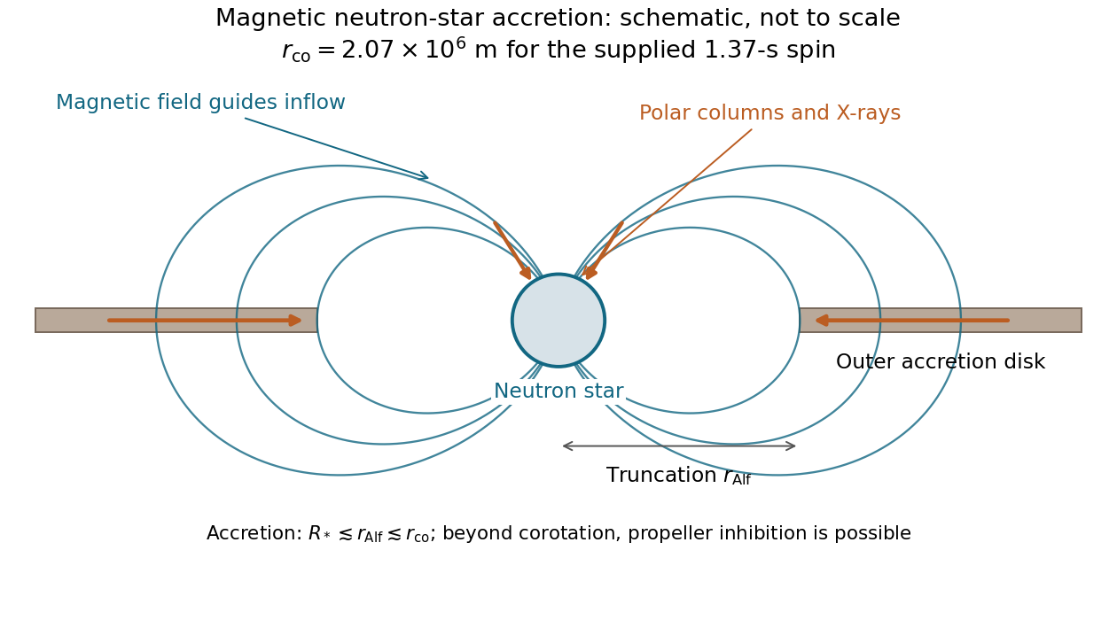
Magnetic channeling from a truncated accretion disk to neutron-star polar caps, with the corotation condition shown separately
. Details. Let yr. With constant moment of inertia, the observed positive spin-up torque isNearly Keplerian material at the inner disk carries specific angular momentum . Equating its inflow rate to the observed torque givesIn the surface accretion Eddington rate convention,The printed coefficient is therefore recovered at its intended approximate precision. This is a material-torque model; magnetic torques, wind angular-momentum loss and a changing stellar moment of inertia are not included.
The accreting-pulsar luminosity and material-torque consistency test shows a concrete tension between the simplest isotropic luminosity estimate and the material-torque estimate. Making their rates equal requiresAn exterior accretion Alfvén radius cannot lie inside a 10-km star. Even taking its smallest exterior value, , the observed torque permits only about in this model, below the isotropic estimate. The discrepancy is modest enough to be sensitive to the approximate radius and moment of inertia, but it prevents claiming exact simultaneous agreement under the stated central values.
Near corotation, the torque gives only . If its radiative efficiency is unchanged, beaming into a fraction about of the sky would reconcile that intrinsic luminosity with the apparent isotropic value. The given truncation formula would then require T for a magnetosphere near corotation. Other possibilities include substantial opposing magnetic torque, outflows separating the disk supply rate from the surface rate, a different radiative efficiency and magnetically altered opacity. These are changes to the elementary model that need independent evidence, rather than a license to use an unphysical truncation radius. Coherent pulsations already identify the accretor as a neutron star; they do not by themselves choose between these accretion-flow refinements.
Use and a spatially flat background dominated by the stated perfect fluid, so . In Newtonian gauge, the scalar energy and momentum constraints from the linearized Einstein field equations combine to eliminate the potential's time derivative and give the stated relativistic Poisson constraint. Its source contains the velocity correction to the coordinate density perturbation. On sub-horizon scales that correction is small for the ordinary growing modes, recovering the Poisson equation for Newtonian gravity; near or outside the horizon the gravitational field cannot be sourced by alone. Equality of the two metric potentials also assumes negligible scalar anisotropic stress.
The fluid equations are the linear energy-continuity and momentum-Euler parts of . Here is the relevant dimensionless sound-speed squared in the adopted fluid closure; for a constant- adiabatic barotropic fluid it equals . A fluid with entropy perturbations needs additional pressure information. The equations actually use in Fourier space, the peculiar-velocity divergence. Calling it simply momentum density is imprecise: it is the divergence of the velocity, with momentum weighted by before normalization. In particular must have inverse-conformal-time units for the displayed continuity equation to be dimensionally consistent.
For the shifted density perturbation in Newtonian gauge, set . The radiation continuity equation gives , and its Euler equation givesWriting , the relativistic constraint becomesEliminating the potential therefore givesThis has the requested . Well inside the sound horizon, , the potential contribution is suppressed relative to the density term and . ThusThese are sound waves: radiation-pressure gradients restore a compression, while inertia carries the fluid through equilibrium. The perfect-fluid approximation neglects diffusion damping and freely streaming species' anisotropic stress. It gives the high-frequency limiting oscillations, not a claim that every radiation-era perturbation is an undriven sinusoid at horizon entry.
For pressureless matter, obeys . The Euler equation givesThe constraint is nowConsequentlyFor a matter-dominated flat background, and . On small scales but : the last term must not be dropped with . The equation becomesSince is small relative to the growing density term on these scales, this recovers .
There is a printed error in the requested super-horizon decaying mode. At , and the leading equation is , henceThe printed fails its own equation: for , the left side is at leading order. The decaying solution would instead result from using the radiation-era background in this limiting damping term. Finite- corrections restore terms of relative order and do not repair the wrong leading power.
A power spectrum describes the variance of Fourier amplitudes as a function of wavenumber. In a statistically homogeneous continuum convention,The paper's is the corresponding finite-volume or normalization-suppressed statement. For statistical isotropy only remains. The dimensionless variance per logarithmic interval is , a different quantity.
The response changes around , or : the velocity contribution to the relativistic constraint and the effective growth equation change relative importance across the horizon-scale transition. Large-scale is approximately constant for its regular mode, while short-scale density perturbations grow gravitationally. A smooth initial potential spectrum can therefore acquire a different dependence in the density spectrum. For illustration, a constant matter-era potential gives , so sufficiently small-scale has four additional powers of relative to , while the very large-scale limits have the same power dependence.
This identifies a dynamical transition, not a universal prediction of the primordial spectrum or an exact spectral break at for arbitrary initial data. The familiar late-time matter-spectrum turnover also retains the history of horizon entry around radiation–matter equality; it is not generically tied to the current Hubble scale. Initial conditions and the intervening expansion history are needed for an actual spectrum.
Write for a uniform ambient mass density. Equating mass, length and time dimensions gives , and . Thus the Sedov-Taylor blast wave hasThe dimensionless coefficient depends on the gas's adiabatic index and on whether denotes the shock radius. Solving the similarity profile for a monatomic ideal gas gives , so taking it as unity is an order-of-magnitude approximation rather than an extra dimensional result.
Timed photographs of the 1945 atomic explosion provide a direct scale test: the measured fireball radius follows over the relevant blast-wave interval, and inserting the independently established explosion energy and atmospheric density gives a coefficient of order unity. The published photographic analysis tested the radius-time law and used its normalization to infer an explosion energy of the correct nuclear-test scale. This illustrates both the success and the limits of dimensional reasoning: the power law is fixed dimensionally, whereas the numerical coefficient requires a profile calculation or measured normalization.[ref]
https://doi.org/10.1098/rspa.1950.0050. Part II, photographic radius-time measurements and explosion-energy estimate; the 20–185 m interval tests the predicted similarity scaling
Neglecting the exterior temperature requires a strong shock, , or . The swept-up mass must dominate the initial ejecta for this energy-conserving similarity stage, while radiative losses, gravity, ambient gradients and continuing energy input must be unimportant. A very hot exterior or a late weak disturbance introduces a sound-speed scale and invalidates the cold-upstream similarity assumptions.
Use the local shock rest frame. Let and label upstream and downstream gas, with positive normal speeds through the shock. The unshocked ISM is almost stationary in the stellar frame, so , whereas the shocked gas moves outward at in that frame. For an ideal monatomic gas, ; neglect upstream pressure and enthalpy in the strong-shock limit. Conservation of mass, momentum and energy per unit mass givesPut . The momentum equation gives . Substitution into the energy equation givesDiscarding the unshocked root leavesThe downstream speed in the stellar frame is therefore , not . These conditions describe immediate shock heating; subsequent cooling and evolution behind the front require the downstream flow profile. Cosmic-ray pressure, radiative energy loss inside the shock layer or a different equation of state would alter the compression ratio.
Let the mean particle mass be , with counting total particles so that . The ideal-gas law and the strong-shock pressure give the immediate post-shock temperatureThe robust prediction is . For a transparent numerical convention take , and . ThenFor an ionized mixture with under the same total-particle-density convention, these normalizations become pc and K. The paper does not specify composition or whether its quoted density instead counts hydrogen nuclei; that convention must be stated, not hidden in a precise age.
The ambient-temperature limit of an adiabatic blast wave gives a formal matching estimate, K, givesWith the age is about yr and the radius stays about 90 pc. This matching criterion already lies outside a very strong shock: in the strong-shock formula corresponds to . A separate sonic estimate gives about yr and 133 pc for ; neither extrapolation is a precise transition solution. Using increases these inferred matching ages and radii by factors .
In a real supernova remnant, substantial radiation losses commonly end the energy-conserving phase before these formal pressure-merging limits. The relevant comparison is against the expansion time. A cooling function, composition and ionization state are needed to calculate that earlier age and radius; they are not supplied. The numerical values above answer the ambient-temperature breakdown estimate under explicit assumptions and must not be presented as a uniquely determined radiative shell-formation age.
After cooling, an interior-pressure-driven shell can approximately follow while pressure remains important. In the limiting momentum-conserving stage, and give . Ultimately ambient pressure and turbulent motions make the disturbance merge with the ISM. These slower stages respect the reduced energy budget rather than continuing an adiabatic strong-shock law indefinitely.
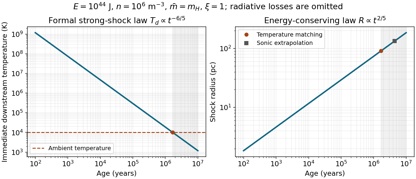
The formal energy-conserving supernova shock temperature and radius, with ambient-temperature and sonic matching distinguished
. Details. A planetary nebula combines a hot post-asymptotic-giant-branch stellar core, its ionized expelled envelope, neutral/molecular material and interstellar dust. Its ultraviolet-to-infrared spectral energy distribution is therefore not a single-temperature blackbody. The principal components are:
- Central-star continuum. A hot stellar photosphere emits strongly in the ultraviolet, especially the ionizing extreme ultraviolet, with its longer-wavelength tail extending through the optical and near infrared. Stellar-atmosphere absorption features and wind lines can be superposed. A companion can add a distinct cool stellar continuum.
- Nebular continuum. Thermal bremsstrahlung, nebular free-bound continuum emission and hydrogen two-photon emission produce a broad continuum. Free-bound edges, especially the Balmer discontinuity at 364.6 nm and the Paschen discontinuity near 820 nm, can be apparent. Hydrogen two-photon decay redistributes the Ly-alpha transition energy into a continuum of pairs rather than one 121.6-nm photon.
- Gas emission lines. Hydrogen and helium recombination lines include H-alpha, H-beta and He II 468.6 nm. Collisionally excited lines of metal ions can dominate individual bands: examples include optical [O III] 495.9/500.7 nm and [N II] 654.8/658.3 nm, ultraviolet C III] near 190.9 nm, and infrared fine-structure transitions such as [Ne II] 12.8 micrometres. A broad-band photometric peak may therefore be a line rather than continuum.
- Dust emission and solid-state structure. Grains absorb stellar/nebular radiation and reradiate it as a broad infrared continuum, often from a distribution of temperatures of order tens to hundreds of kelvin; compact hot dust can add near-infrared emission. Carbon-rich material may show aromatic bands around 3.3, 6.2, 7.7, 8.6 and 11.3 micrometres, while oxygen-rich material may show silicate features near 9.7 and 18 micrometres. These are compositional alternatives, not mandatory features of every nebula.
- Neutral and molecular emission. Surviving molecular material in dense clumps or a photodissociation region can contribute infrared rotational/rovibrational lines, notably molecular-hydrogen emission such as the 2.12-micrometre line. Shocks as well as ultraviolet pumping can excite it. Colder dust continues into the far infrared, and low-lying CO rotational lines extend the overall spectrum into the submillimetre/millimetre range.
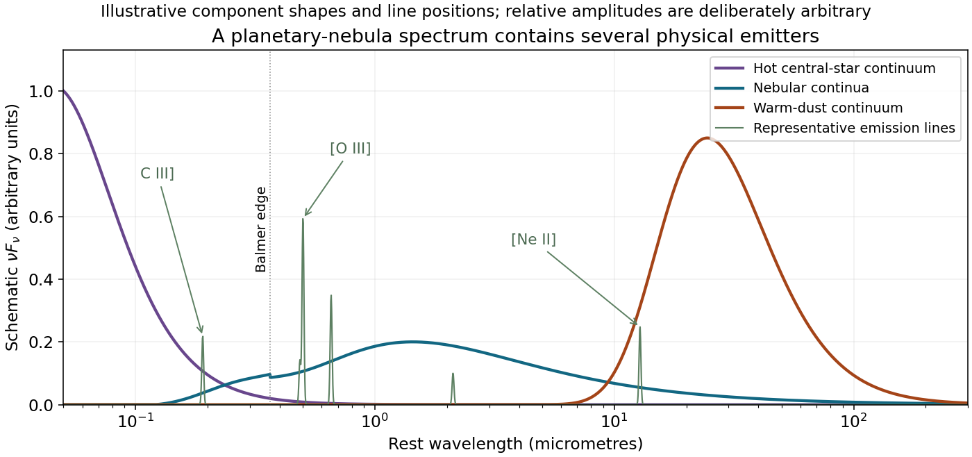
Schematic stellar, nebular and dust components of a planetary-nebula spectrum; arbitrary relative normalizations
. Details. The observed mixture also contains attenuation by internal and foreground interstellar extinction. A spectrum containing all these components need not spatially coincide: stellar light, ionized gas, dusty clumps and the molecular envelope sample different regions.
Stellar radiation and nebular ionization. The planetary-nebula spectral energy distribution is constrained by a shared radiation and thermal balance. The central star's effective temperature, luminosity and evolutionary state set its continuum and ionizing-photon supply. A hotter star shifts the ionizing spectrum and allows higher ionization stages; the total recombination output also depends on how many ionizing photons the gas actually absorbs. In an ionization-bounded nebula, approximate photoionization balance iswhereas a density-bounded nebula can leak photons. Dust absorption of ionizing photons changes this relation further. Stellar-atmosphere and wind effects make a blackbody an approximation, especially in the extreme ultraviolet. A changing core temperature and expanding envelope explain why nebular spectra evolve.
Nebular continua and recombination lines. Their strength depends on the emission measure, roughly , electron temperature, ionic abundances and radiative branching probabilities. For a recombination line,Case-B line ratios assume appropriate trapping of Lyman-series photons and escape of the lower-series radiation. Density, optical-depth effects and extinction can alter observed ratios. The free-free emissivity has the schematic dependence ; the nebular free-bound continuum also carries ionization thresholds and recombination cross-sections. Two-photon emission depends on the population of the hydrogen state and can be reduced by collisional mixing into . Density clumping matters because these rates are weighted approximately by density squared, not simply by total gas mass.
Collisionally excited lines. Below a line's critical density of an atomic transition,Elemental abundance, ionic fraction and electron temperature therefore all enter. The ionizing spectrum and local ionization parameter help determine which ion is present. Above the critical density of an atomic transition, collisional de-excitation competes with radiative decay and can suppress a forbidden line. Low-energy infrared fine-structure lines are generally less exponentially temperature sensitive than high-excitation optical/ultraviolet lines. Metal-line cooling also helps set the temperature, so changing an abundance changes both the number of emitters and the thermal balance; line luminosity need not be proportional to abundance at fixed everything else.
Dust and molecules. Nebular dust spectral features identify the carriers as well as contributing to the integrated luminosity. In an optically thin dust component,The grain mass sets its normalization, while the radiation field, stellar distance, grain size and absorption efficiency determine its temperature distribution. For approximately grey heating, radiative equilibrium suggests ; non-grey grains change this scaling. Long-wavelength opacity is often approximated as . Small aromatic grains undergo transient heating, so one equilibrium temperature is not adequate for every infrared feature. Carbon-to-oxygen chemistry, grain processing and shielding affect aromatic versus silicate bands. Molecular line emission further depends on molecule abundance, collisional density, kinetic temperature, ultraviolet pumping and shocks, while shielding and dissociation set whether molecules survive at all.
Finally, interstellar extinction preferentially suppresses ultraviolet and optical light, and dust reradiates some absorbed energy in the infrared. Aperture, angular resolution and distance must be treated consistently before comparing stellar, nebular and dust components. These dependencies make the combined spectrum an energy and abundance diagnostic, but also prevent a unique reconstruction from a single broad-band colour.
Cold molecular hydrogen is difficult to observe directly: its homonuclear symmetry forbids electric-dipole rotational transitions, and its lowest useful quadrupole rotational excitation is high compared with a cold cloud's temperature. Carbon monoxide is relatively abundant, has a permanent dipole moment and has low-lying rotational transitions that can be collisionally excited in cold gas. The low- lines lie in accessible millimetre bands and suffer much less dust extinction than visible light. They therefore reveal molecular-gas velocities and spatial structure efficiently.
The advantages do not turn CO into a direct mass counter without a model. Common-isotope lines can be optically thick; excitation can be subthermal or have multiple temperatures. Abundance changes with metallicity, chemistry, shielding and photodissociation, and CO can freeze onto grains. Molecular hydrogen can also survive where CO is weak, giving CO-dark gas. A calibrated carbon-monoxide tracer of molecular hydrogen conversion may be useful for appropriate cloud populations but should not be transplanted uncritically to newly formed supernova ejecta. The line calculations here infer CO mass, not total molecular mass unless a CO-to-hydrogen abundance is separately known.
Assume a single-temperature optically thin local thermodynamic equilibrium population, negligible line absorption/stimulated corrections, and that the measured line luminosity is from the remnant's CO. Each spontaneous decay emits , givingFor a rigid rotor, with K. The degeneracy is , and the rotational partition function isAt 20 K the direct sum gives , ; the approximation is already adequate. Thus, with molecular mass ,The remnant age does not enter this optically thin population count. It becomes relevant when estimating emitting volume, density, expansion and optical depth to test the assumptions.
For optically thin CO rotational thermometry of the same emitting population, the upper-level abundance ratio isThe difference can be obtained directly from the two successive transition frequencies, , or approximately from . Using the supplied rounded molecular data gives K. ThereforeThe observed ratio is , henceAt 20 K the predicted ratio would be only about 61, so the two detections reject that single-temperature optically thin 20-K model. The inferred value is an excitation temperature under the stated assumptions, not a model-independent measurement of the gas's kinetic temperature.
Raising the temperature populates higher rotational states and reduces the fraction in . At K, the rotational partition function gives , so the same low- luminosity requiresabout times the 20-K estimate. Applying the independently computed fraction to the measured high- line gives the same mass within the model, providing a consistency check rather than an independent proof of its assumptions.
Optical depth, density-dependent excitation, multiple temperature components, beam dilution, aperture mismatch, line blending and flux calibration all need investigation. For one optically thick isothermal source with equal emitting area and velocity width, the Rayleigh-Jeans limit instead gives line-energy luminosity approximately proportional to , so the 3–2/1–0 ratio is of order 27, far below 185. That illustrates why optical-depth and emitting-area assumptions cannot be ignored; different source areas or excitation structures can change this simple comparison. Optically thick clumps can hide mass, and a high-temperature component may dominate the 3–2 line while colder material contributes much of the 1–0 emission.
Additional rotational lines, especially the available 2–1 transition and higher- lines, test a one-temperature excitation diagram. Less abundant isotopologues help constrain opacity; resolved imaging and line profiles constrain emitting volume and homologous expansion, using the remnant age. Density information permits non-LTE statistical-equilibrium/radiative-transfer modelling. Dust emission can provide a complementary mass constraint with its own opacity and dust-to-gas uncertainties. A total gas mass additionally needs a justified CO abundance, accounting for molecular formation, destruction and unobserved material.
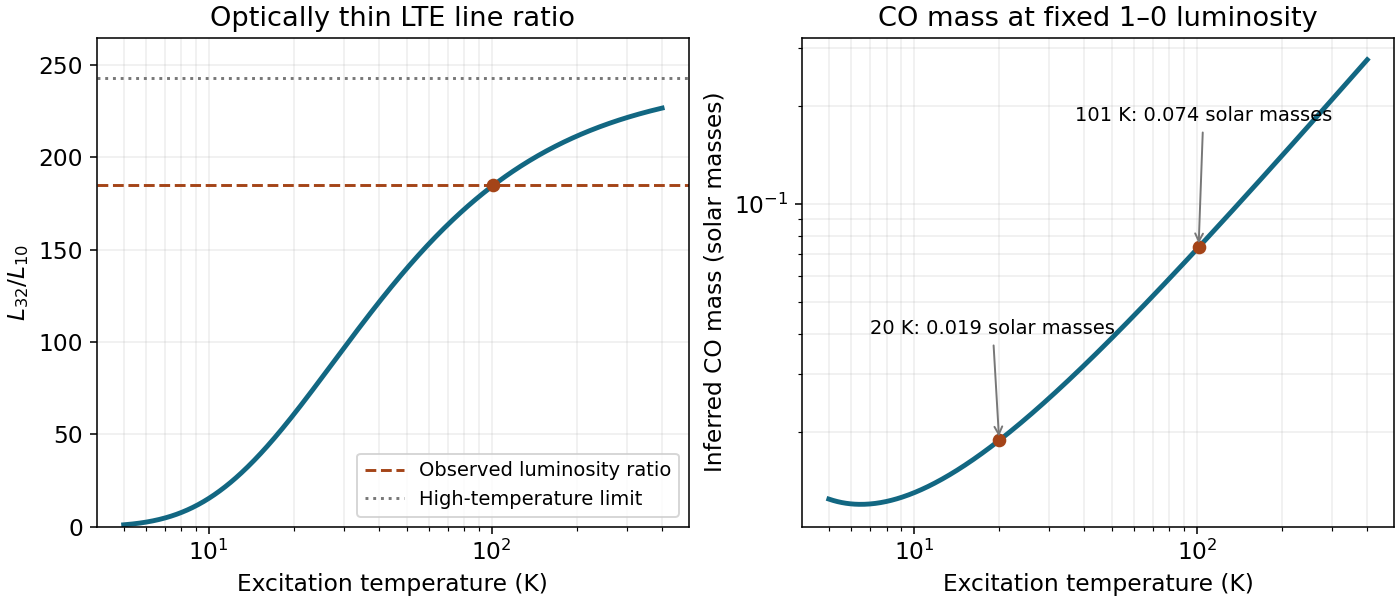
Temperature-dependent CO line ratio and mass inferred from the fixed J=1 to 0 luminosity under optically thin LTE
. Details. For a steady spherical, nonrotating, bounded collisionless galaxy, the mean velocity vanishes, the mixed velocity moments vanish, and . A steady radial stellar flux would satisfy ; regularity and no central source/sink set that constant to zero in the equilibrium model. The Spherical Jeans equation is thereforeHere is the tracer number density, not necessarily the gravitating mass density. Random motions supply the velocity stress balancing the gravitational field.
Two conventions in the printed general equation need correction before interpreting it outside this special limit. Its first standalone derivative of mean radial velocity should be a time derivative, , not : the latter has incorrect acceleration dimensions. Also a velocity dispersion is the centered moment . The printed raw-moment definition equals it only when the mean velocities vanish, as they do in the equilibrium used here. These issues do not change the simplified result above.
For an ensemble of nearly circular stellar orbits with randomly oriented planes, radial motion is small while tangential motion is substantial: . The two tangential variances remain equal by spherical symmetry. There need not be bulk rotation even though individual stars move on nearly circular paths. The anisotropy parameter is strongly negative; its exactly circular limit is singular as .
Nearly radial orbits have small transverse motion: . A bounded steady population contains both inward and outward phases, so large radial dispersion is compatible with zero mean radial velocity. Positivity of the distribution function and stability can impose further restrictions on particular radial models.
An isotropic velocity distribution has equal variance in every direction and zero mixed moments:This is a statement about random velocity directions at each radius, not a requirement that every star follows a circular orbit.
For spherical gravity, . Inserting into the Spherical Jeans equation and solving for the total enclosed mass givesThe mass includes all sources of the potential, including dark matter or a central compact object; the stellar tracer density need not follow total mass. The bracket must yield nonnegative enclosed mass in a physically admissible model. Density, radial stress and anisotropy are independent observational/model inputs before this equation becomes a mass estimate.
TODO: the original line-of-sight geometry figure on source page 8 is unavailable. The PDF calls an unembedded image and the documented archive parent has the same gap. Its exact drawn layout cannot be checked or reproduced. The surviving coordinate definitions suffice for the following standard spherical-projection derivation; no missing plotted values or drawn dimensions are supplied here.
The spherical density projection schematic below is original geometry constructed from these definitions, not a recovered examination figure.
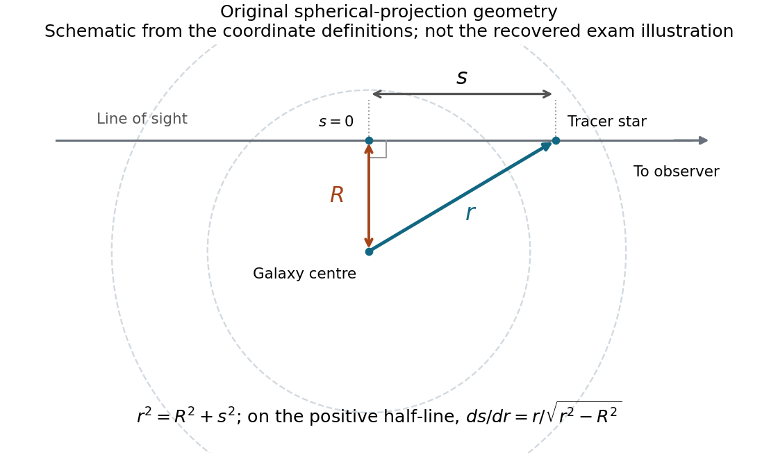
Original line-of-sight geometry from the surviving coordinate definitions; not the recovered examination figure
. Details. Let be closest approach on a line of sight at projected radius . Euclidean spherical geometry gives . On either half-line, , and the two halves contribute equally. With identical stellar luminosity , , soFor an isotropic velocity distribution, the variance of any unit-direction projection equals . Explicitly, the line-of-sight contributions have weights from the radial component and from a tangential component; equality of their variances makes the sum . ConsequentlyWithout isotropy the integrand instead has the factor . Thus the projection assumption is substantive, rather than something that can be inferred from spherical surface brightness alone. The missing illustration does not prevent recovering these algebraic expressions from the prose.
For the isotropic Jeans-Abel mass inversion, let and . The two preceding projections have the same Abel integral equation kernel, givingTheir ratio recovers , and the isotropic Jeans equation givesEquivalently put and . Then : the common stellar luminosity cancels from the inferred mass. Differentiating these singular-kernel integrals is understood through suitable regularity or a nonsingular variable change, not by naively keeping an infinite lower-end boundary term.
The inversion assumes adequate radial coverage, convergence and a smooth spherical equilibrium. In practice derivatives amplify noise and the unobserved outer tail needs treatment or a model. Unknown anisotropy reintroduces a mass–anisotropy degeneracy; the uniqueness just derived is conditional on the explicitly isotropic velocity distribution.
Use the supplied comoving distance Mpc. In a flat background, Mpc and Mpc. The observed wavelength is stretched by , soCare is needed with a luminosity per frequency. For corresponding emitted and observed frequencies, . Combining that bandwidth relation with the bolometric definition of givesThis is the spectral luminosity at the rest-frame frequency corresponding to 200 nm. A value at some different rest wavelength would require the quasar's spectral shape. The factor is different for a density per unit wavelength; interchanging these two conventions would give an incorrect redshift factor.
A transverse physical size is angle times angular diameter distance, not luminosity distance or comoving distance. Converting the apparent diameter into radians givesThis is the galaxy's projected proper diameter at the emission epoch. Its corresponding comoving diameter is three times larger.
The projected quasar-to-cloud separation isFor the usual transverse-separation estimate, take the cloud to lie at the same line-of-sight proper distance as the quasar. Since the cloud and galaxy are gravitationally bound, the local source-to-cloud path does not acquire the redshift factor that separates that system from us. Neglect internal relative Doppler shifts and attenuation. The observer in the cloud seesThis uses the quasar's isotropic intrinsic emission at the same rest frequency; anisotropic radiation or obscuration would modify it.
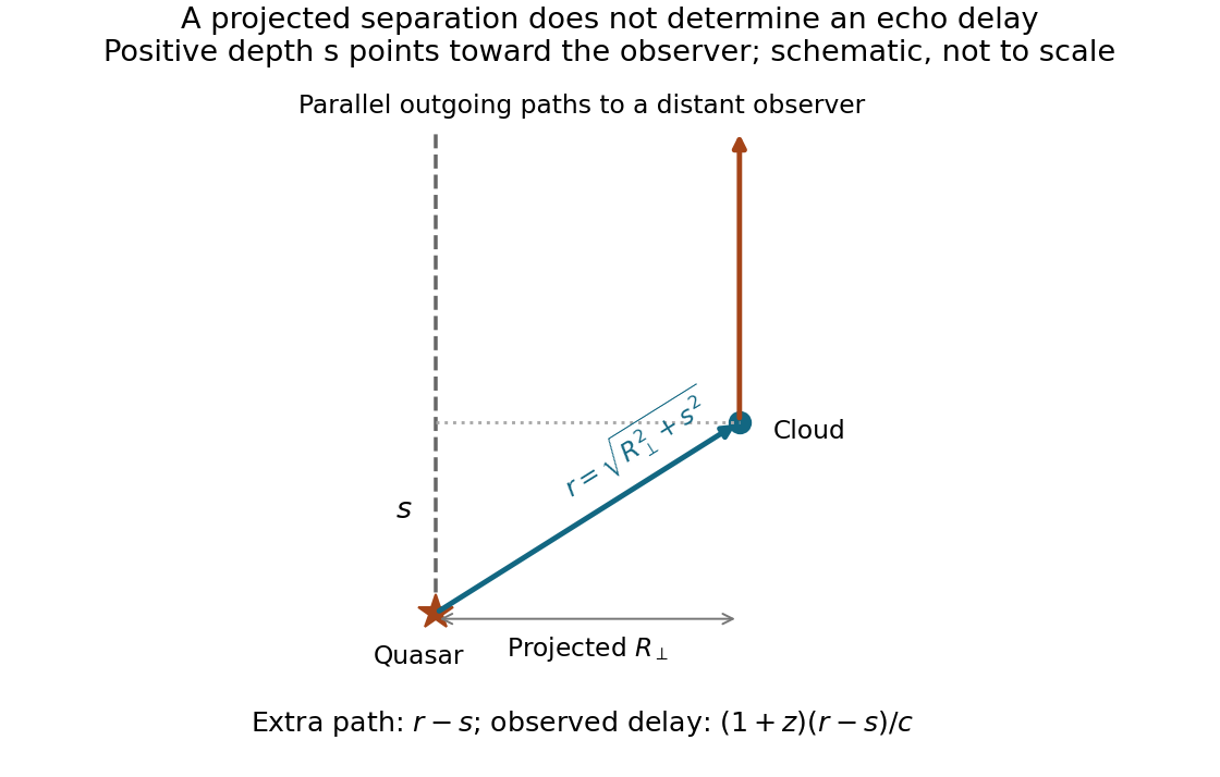
An angular separation only fixes . If is a source-to-cloud displacement toward us, the true local distance is and the general flux is . The quoted transverse value is therefore an upper estimate at fixed projected separation. Equality of cosmological redshift and gravitational binding do not by themselves measure the small internal line-of-sight displacement; a peculiar velocity can also mask it.
For a bound-cloud light echo, the relevant observed delay is the excess source–cloud–observer path over the direct source–observer path, with the interval dilated by cosmological expansion. For a cloud displaced by toward us,The formula assumes source and cloud separation is small compared with their cosmological distance, so their distant observer directions are effectively parallel. For the transverse configuration ,The local quasar-to-cloud travel time is about yr; the factor three is needed for the interval measured by us. A foreground cloud shortens the echo delay and a background cloud lengthens it. A unique value beyond this transverse estimate needs the otherwise unspecified depth, even if the cloud's intrinsic response is instantaneous.


For a small peculiar line-of-sight velocity within the group, cosmological and Doppler factors multiply:At fixed group redshift this gives . ThereforeUsing directly would give a detector-frame redshift interval without removing the cosmological stretch. This is the one-dimensional line-of-sight velocity dispersion requested, not the three-dimensional RMS speed. Redshift measurement errors or a large unbound line-of-sight extent would require additional corrections; neither is supplied here.
For a transverse comoving separation Mpc in a flat universe, the corresponding distance is the transverse comoving distance , soEquivalently the physical separation is Mpc and dividing it by Mpc gives the same angle. Dividing 100 comoving Mpc directly by would mix scale conventions. The density's Mpc is a characteristic inter-object spacing; a particular nearest neighbour has a distribution of distances and orientations.
For a small radial comoving interval, . At ,ThusThis uses the unbound cosmological radial separation between separate quasars, unlike the peculiar-velocity redshift dispersion of galaxies inside the bound group. Integrating the distance relation instead of linearizing gives a small correction for a specified direction and endpoint. The quoted characteristic spacing alone does not assert that the same nearest object lies both purely transverse and purely radial.
Articles by others on the same topic
There are currently no matching articles.