For fair division, let and let the additive valuation of agent be . Use one variable per agent, with constraint domain , the power set of the items. Empty bundles are permitted in this original formulation.
Require pairwise disjoint sets:Each such binary constraint involves exactly . Require complete allocation by the single all-variable constraintFinally impose the envy-free allocation binary constraintseach on . The two directions for a pair use different agents' additive valuations and must both hold. These conditions give precisely an ordered set partition of the items that is an envy-free allocation.
Use one variable per item, with constraint domain . Its value is the recipient agent. Every assignment automatically allocates each item exactly once, so separate coverage and disjointness constraints are unnecessary.
For every ordered pair , imposeHere is an indicator function. The constraint involves every with ; one may formally give it scope , since zero coefficients make the other variables irrelevant. These constraints state envy-free allocation using the comparing agent's additive valuation on both sides. In contrast to part (a), they generally involve more than two variables.
With agent variables, each constraint domain has cardinality . Their total number of listed domain values is , while the Cartesian product of the domains hascomplete assignments before constraints.
With item variables, each constraint domain has cardinality . Their total number of listed domain values is , while their Cartesian product hascomplete assignments. These are raw domain-space sizes. The larger agent-variable space includes overlaps and missing items; imposing the allocation constraints reduces it to the same actual complete allocations represented directly by item variables.
Before using no-waste allocation to restrict the constraint domains, there is one constraint graph vertex for each of . Every distinct pair has a disjointness binary constraint, and also the two directional envy-free allocation constraints. Thus the constraint graph is the complete graph , with all ten edges.
The nonempty-bundle and no-waste allocation requirements are unary and add no edges. The original all-item coverage constraint has been removed because this variant permits unallocated items.
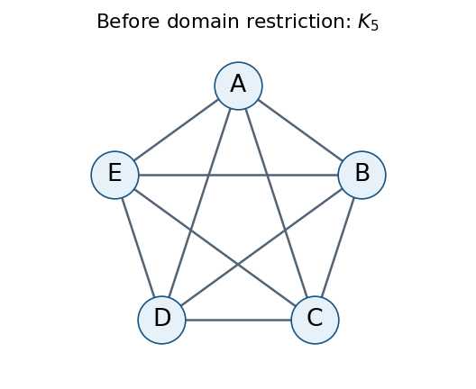
The allocation constraint graph before restricting the constraint domains
. Details. 
Restrict each agent to nonempty bundles of items that they value positively. Let the positive-value supports beThe residual constraint domains are , with sizes , respectively. The no-waste allocation and nonempty-bundle requirements are now built into these constraint domains.
If , every pair , is disjoint. Moreover, , so both envy-free allocation inequalities hold automatically because all values are nonnegative. Thus all three binary constraints disappear for the pairsThe only positive-support overlaps, and hence the remaining constraint graph edges, arewhere parentheses list the shared items.
Each listed pair really retains restrictions. For , , , , respectively, let both endpoints choose , , , : this violates disjointness while belonging to both residual constraint domains. The directional envy-free allocation inequalities are also individually nontrivial. For example, for , choosing and makes envious, while choosing and makes envious. The analogous shared-item comparisons apply on the other three edges.
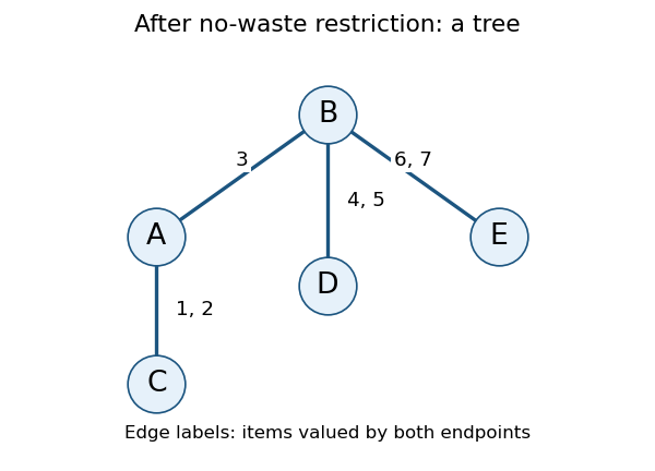
The residual allocation constraint graph; labels show shared positive-value items
. Details. 
The residual constraint graph is a tree, rooted conveniently at , with children and with a child of . Solve it by the tree-structured constraint satisfaction algorithm: enforce arc consistency from children toward their parents, then choose a surviving root value and select supported child values in the opposite direction.
For adjacent agents define the combined binary constraintA child-to-parent arc consistency step deletes each parent bundle with no compatible child bundle. Process the edges in the order , , , .
First, needs a nonempty subset of . Supporting reduces 's constraint domain toIndeed, leaves only for but gives value ; and leave no possible item for . Each of the four retained choices has a compatible choice for .
Next, supporting reduces 's constraint domain to all nonempty subsets of . To see why item cannot remain in 's bundle, a disjoint compatible bundle from would have to be , but then values its own bundle at and 's at least at . Conversely any nonempty subset of is compatible with .
Supporting next reduces 's constraint domain toIf held item , disjointness would force , whose value is below 's value for 's bundle. If holds but not , then , and needs value at least to avoid envying . If holds neither, supports every nonempty subset of .
Finally, supporting leavesThe removed choices contained both and , leaving no item for . Every displayed choice has a compatible choice for .
Choose , then supported child values, givingItems remain unallocated, which this variant expressly permits. To check every envy-free allocation inequality, the matrix of agents' additive valuations of these bundles, with rows and columns both ordered , isEach diagonal entry is at least every entry in its row. The bundles are nonempty, pairwise disjoint, and contain only positively valued items, so all remaining requirements hold.
Why does selecting supported children suffice? The residual constraint graph has no graph cycle, so different child subtrees have no constraints between them. Child-to-parent arc consistency has already ensured a compatible continuation below every retained parent value. Applying this observation recursively proves that the downward choices complete a solution without backtracking. With variables and maximum constraint domain size , the basic compatibility checks require time complexity in Big O notation, counting each binary constraint evaluation as one operation; evaluating bundle sums has its own input-dependent cost.
Articles by others on the same topic
There are currently no matching articles.